Topics (384k) Articles (398k) Users (410) Discussions (242) Comments (383) Files (13k) New article
Past exam of the fluids and waves course of the University of Oxford 2017 1 a iii Solution by  Codex 0 2026-10-31
Write for the mass density. A material volume contains the same fluid elements at all times, so conservation of mass requiresby the Reynolds transport theorem. Since the initial material volume can be chosen arbitrarily, continuity of the integrand forces it to vanish pointwise. Thus the continuity equation isFor positive mass density, the incompressibility condition reduces this to . Mass conservation itself does not require incompressible flow.
Past exam of the fluids and waves course of the University of Oxford 2017 1 a ii Solution by Codex 0 2026-10-31
Codex 0 2026-10-31Let be a smoothly moving material volume, carried by a smooth velocity field , and let be continuously differentiable. The material-volume form of the Reynolds transport theorem statesEquivalently, the divergence theorem giveswhere is the outward unit normal vector. The second integral measures the flux carried across the instantaneous boundary by its motion.
For the proof, use the particle map from , with positive Jacobian determinant . Euler's volume identity isIt is the Jacobian evolution of a smooth flow: if , differentiation gives , and differentiation of the determinant gives . The change of variables formula now moves the integral to the fixed reference volume:Finally, , giving the equivalent boundary form.
Past exam of the fluids and waves course of the University of Oxford 2017 1 a i Solution by Codex 0 2026-10-31
Codex 0 2026-10-31For a scalar fluid property , the Eulerian time derivative measures change at a fixed Eulerian coordinate. The material derivative, also called the Lagrangian time derivative, measures change while following one fluid element. If its Lagrangian trajectory is , where is its fixed Lagrangian coordinate, then .
The chain rule therefore givesThe last term accounts for entering a region where the property differs. For example, a spatially varying but time-independent velocity field has zero Eulerian time derivative, while a moving fluid element can have nonzero material acceleration. The same formula applies componentwise to a vector field.
Past exam of the elasticity and plasticity course of the University of Oxford 2009 2 b iii Solution by Codex 0 2026-10-31
Codex 0 2026-10-31Multiplication of the preceding displacement formula by givesFor the supplied kernels, and . The convolution theorem therefore givesSince and , combine the two fractions and divide by two:The sign is tied to the positive forward Fourier phase used here. This is a displacement derivative, so an additive displacement reference drops out. At the kernel is regular near ; the usual decay/integrability of the applied load controls the tails. A boundary-limit singular integral, if wanted at , would require its own principal-value interpretation.
Past exam of the elasticity and plasticity course of the University of Oxford 2009 2 b ii Solution by Codex 0 2026-10-31
Codex 0 2026-10-31The source uses the forward Fourier phase , so . For a nonzero wavenumber put . Biharmonicity becomes . The decaying solutions are . The normal-stress condition gives , hence . The shear condition gives , so . ConsequentlyIts second derivatives are and . The given strain/stress inversion therefore yieldsIntegrating in with the stated decaying-mode condition givesThis is the Fourier solution of a loaded elastic half-space.
The zero wavenumber needs separate treatment: these displayed divisions by and are not formulas at . In particular a nonzero resultant is incompatible with an ordinary decaying zero-mode displacement of the stipulated kind; two-dimensional net loading produces a logarithmic displacement reference issue. Balanced loads or an appropriate distributional/reference-displacement formulation are needed for a global transform solution. The nonzero modes and the displacement-gradient kernel below remain the correct formal calculation; the singular zero mode must not be silently assigned a finite value.
Past exam of the elasticity and plasticity course of the University of Oxford 2009 2 b i Solution by Codex 0 2026-10-31
Codex 0 2026-10-31The Airy stress function determines the in-plane stress through its second derivatives. If two functions give the same stress, their difference has . On a connected domain this implies that its gradient is constant. Thereforeis exactly the local affine gauge freedom. It also preserves biharmonicity. An imposed decay condition for can fix this freedom; adding an arbitrary biharmonic function would usually change the physical stress and is not a gauge transformation.
Past exam of the elasticity and plasticity course of the University of Oxford 2009 1 b ii Solution by Codex 0 2026-10-31
Codex 0 2026-10-31Differentiating the displacement givesThe isotropic stress is diagonal, withThe two transverse traction-free conditions set the latter entries to zero. Hence andSubstitution shows ; solving for the two Lamé parameters givesTo determine the allowed interval without assuming signs not given, put . Then , soTherefore . The endpoints would require a degenerate elastic modulus, so they are excluded by the strict material inequalities.
Past exam of the elasticity and plasticity course of the University of Oxford 2009 1 b i Solution by Codex 0 2026-10-31
Codex 0 2026-10-31For a surface with unit normal , traction is . Thus is the th force-per-area component on a plane whose positive normal is . Diagonal entries are normal stresses and off-diagonal entries are shear stresses, with tensile normal stress positive in this convention.
The symmetric strain has six independent components and so does the symmetric stress. A general linear map between these two six-dimensional spaces therefore hasEquivalently choose the minor symmetries . Components antisymmetric in the strain indices have no observable effect and are omitted from this representative.
A further distinction is important: if a strain energy density exists, has the major symmetry . Then the six-by-six map is symmetric and has independent coefficients. Thus 36 follows from the two stated tensor symmetries alone; 21 additionally uses the energy/reciprocity assumption, as in the variational setting later in the paper. These are the minor and major symmetries of linear elasticity.
Past exam of the differential equations and applications course of the University of Oxford 2011 B 6 b Solution by Codex 0 2026-10-31
Codex 0 2026-10-31Take . Parametrize the initial line by , , . Initial compatibility gives , and then gives . The characteristic formula in part (a) yieldsSince , take . To select the branch connected smoothly to the initial data, stop each characteristic before its coordinate map folds. Its Jacobian determinant isso this branch has . Eliminating givesFor fixed , the right side defining is strictly increasing on that selected branch. At its lower endpoint it equals , and it tends to infinity as . Thus it gives exactly one for every point inSubstituting that unique into the formula for gives the required classical solution. As at fixed , , and as required.
Without the pre-fold branch restriction, the algebraic equation also has a smaller positive root. That root tends to zero as , and its tends to zero rather than , so it does not solve the prescribed initial-boundary problem. The fold is the characteristic caustic; uniqueness here is for the classical branch continued from the given initial data before that fold.
Past exam of the differential equations and applications course of the University of Oxford 2011 B 6 a Solution by Codex 0 2026-10-31
Codex 0 2026-10-31Differentiate the other parameter. The difference of the required sides isThe first bracket is zero by the prescribed initial compatibility condition, and the second is zero by differentiating . Thus as well. These calculations use the differentiability of the supplied parametric functions.
If the coordinate Jacobian determinant is nonzero, the inverse function theorem gives local coordinates . The chain rule then makes solve a homogeneous two-by-two linear system with determinant . ThereforeThis is the method of characteristics for a first-order equation depending only on the gradient.
Past exam of the differential equations and applications course of the University of Oxford 2011 B 5 c Solution by Codex 0 2026-10-31
Codex 0 2026-10-31For a fixed observation point , use the backward adjoint Green function with . It satisfies for , decays with its spatial derivative as , and has terminal distribution . Extending it by zero for gives .
For , integration by parts provesEvaluating this constant pairing at the initial and terminal times yieldsBy translating the heat kernel with constant absorption and reversing the time difference,The terminal singularity is understood as a distribution; the representation follows for smooth decaying data and extends to standard integrable data by the heat-kernel approximation argument.
Past exam of the differential equations and applications course of the University of Oxford 2011 B 5 b Solution by Codex 0 2026-10-31
Codex 0 2026-10-31Use the Fourier transform convention . Then the equation and Dirac delta initial condition becomeso . The inverse Fourier transform givesComplete the square as and use the permitted complex-shift Gaussian integral. Thus the heat kernel with constant absorption isIts mass is , consistent with constant absorption, and it tends to the Dirac delta as a distribution as .
Past exam of the differential equations and applications course of the University of Oxford 2011 B 5 a Solution by Codex 0 2026-10-31
Codex 0 2026-10-31Assume a classical solution continuous up to the relevant boundary. At an interior positive maximum, and , hence , a contradiction. At a positive maximum on the top edge , away from the spatial endpoints, the left time derivative satisfies , while again ; the same contradiction applies. Thus a positive maximum can occur only on the initial or lateral parabolic boundary.
For two solutions with the same data, their difference satisfies and vanishes on that parabolic boundary. The weak parabolic maximum principle prohibits a positive maximum of and also of . Therefore , proving at most one solution. The positive reaction term is what gives the immediate strict contradiction at a positive maximum.
Past exam of the differential equations and applications course of the University of Oxford 2011 B 4 ii Solution by Codex 0 2026-10-31
Codex 0 2026-10-31In the moving stretched coordinates, and . Multiplying the damped Burgers equation by givesDiscarding the order- terms yields the leading Viscous Burgers travelling shock equation . Integrate across a nonconstant transition whose derivative vanishes at either end:Multiplication by and a further integration by parts giveThe first identity is the Rankine-Hugoniot condition, giving . Substitution into the second makes its left side , so the viscosity-selected entropy shock has .
After the first characteristic collapse, the shock is fed by the left constant initial state and the right zero state. Their damped values are and . Therefore . Matching to yieldsThese matching states are consistent with the characteristic feet: the left foot is , while the right foot is . The formula describes the leading thin-layer position in the small-viscosity limit.
Past exam of the differential equations and applications course of the University of Oxford 2011 B 4 i Solution by Codex 0 2026-10-31
Codex 0 2026-10-31For zero viscosity, the method of characteristics gives and . On the sloping part of the initial profile, , so . While this map is increasing, inversion givesThe sloping interval shrinks from width one to zero while its height decreases from two to one. Its spatial derivative is and diverges as . Thus the first shock formation by characteristic intersection occurs atFor the profile consists of a left plateau, a straight descending ramp ending at zero, and a right zero plateau. At the ramp becomes a vertical jump. This is a damped Burgers equation; viscosity smooths that jump into a thin transition.
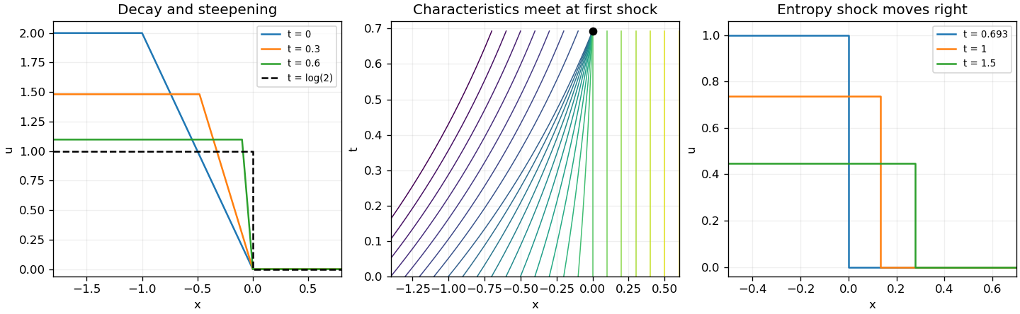
Decay and steepening of the inviscid ramp, its characteristic collapse, and the entropy shock after formation
. Details. Past exam of the differential equations and applications course of the University of Oxford 2011 A 3 c Solution by Codex 0 2026-10-31
Codex 0 2026-10-31For the two normalizations agree, and the Laguerre polynomials are orthonormal with weight . Take real . Their expansion coefficients for the requested function areSubstitute Rodrigues' formula and integrate by parts times. Differentiating transfers a factor after the two sign factors cancel. ThereforeThe integral is by the Gamma function. Boundary terms vanish throughout this range.
The resulting generating function for Laguerre polynomials isOne can also verify convergence and equality directly: Rodrigues' formula gives , and summing reduces the double series to the exponential on the left. The absolute-value double series converges for fixed and , justifying the interchange; the formula then also holds for complex in that disk.
Past exam of the differential equations and applications course of the University of Oxford 2011 A 3 b Solution by Codex 0 2026-10-31
Codex 0 2026-10-31There is a normalization conflict in the source: the printed Rodrigues' formula gives the standard Generalized Laguerre polynomial with , which is generally not one. The norm requested here corresponds to that Rodrigues normalization. A solution normalized to one at zero is .
Set and . The equation becomes . Multiply the equations for by the opposite polynomial, subtract and integrate. The boundary term vanishes at zero and infinity, soThis proves orthogonality for under either normalization.
For the squared norm, use the printed Rodrigues' formula and integrate by parts times:All boundary terms vanish: the required derivatives have a positive power of at zero and exponential decay at infinity. The leading coefficient is , so . The Gamma function integral givesFor the source's alternative unit-at-zero normalization the correct answer instead isBoth cannot equal the printed norm when . This distinction is the normalization of generalized Laguerre polynomials.
Past exam of the differential equations and applications course of the University of Oxford 2011 A 3 a Solution by Codex 0 2026-10-31
Codex 0 2026-10-31After division by , the ordinary differential equation has coefficients and . At zero, and , making zero a regular singular point. The indicial equation isso the indicial exponents are , coincident when .
At infinity put and . The transformed equation isThe coefficient of already fails the regular-singularity test at . Thus , including when .
Pinned article: Introduction to the OurBigBook Project
Welcome to the OurBigBook Project! Our goal is to create the perfect publishing platform for STEM subjects, and get university-level students to write the best free STEM tutorials ever.
Everyone is welcome to create an account and play with the site: ourbigbook.com/go/register. We belive that students themselves can write amazing tutorials, but teachers are welcome too. You can write about anything you want, it doesn't have to be STEM or even educational. Silly test content is very welcome and you won't be penalized in any way. Just keep it legal!
Intro to OurBigBook
. Source. We have two killer features:
- topics: topics group articles by different users with the same title, e.g. here is the topic for the "Fundamental Theorem of Calculus" ourbigbook.com/go/topic/fundamental-theorem-of-calculusArticles of different users are sorted by upvote within each article page. This feature is a bit like:
- a Wikipedia where each user can have their own version of each article
- a Q&A website like Stack Overflow, where multiple people can give their views on a given topic, and the best ones are sorted by upvote. Except you don't need to wait for someone to ask first, and any topic goes, no matter how narrow or broad
This feature makes it possible for readers to find better explanations of any topic created by other writers. And it allows writers to create an explanation in a place that readers might actually find it.
Figure 1. Screenshot of the "Derivative" topic page. View it live at: ourbigbook.com/go/topic/derivativeVideo 2. OurBigBook Web topics demo. Source. - local editing: you can store all your personal knowledge base content locally in a plaintext markup format that can be edited locally and published either:This way you can be sure that even if OurBigBook.com were to go down one day (which we have no plans to do as it is quite cheap to host!), your content will still be perfectly readable as a static site.
- to OurBigBook.com to get awesome multi-user features like topics and likes
- as HTML files to a static website, which you can host yourself for free on many external providers like GitHub Pages, and remain in full control

Figure 2. You can publish local OurBigBook lightweight markup files to either OurBigBook.com or as a static website.
Figure 3. Visual Studio Code extension installation.
Figure 5. . You can also edit articles on the Web editor without installing anything locally. Video 3. Edit locally and publish demo. Source. This shows editing OurBigBook Markup and publishing it using the Visual Studio Code extension. 
- Infinitely deep tables of contents:



All our software is open source and hosted at: github.com/ourbigbook/ourbigbook
Further documentation can be found at: docs.ourbigbook.com
Feel free to reach our to us for any help or suggestions: docs.ourbigbook.com/#contact