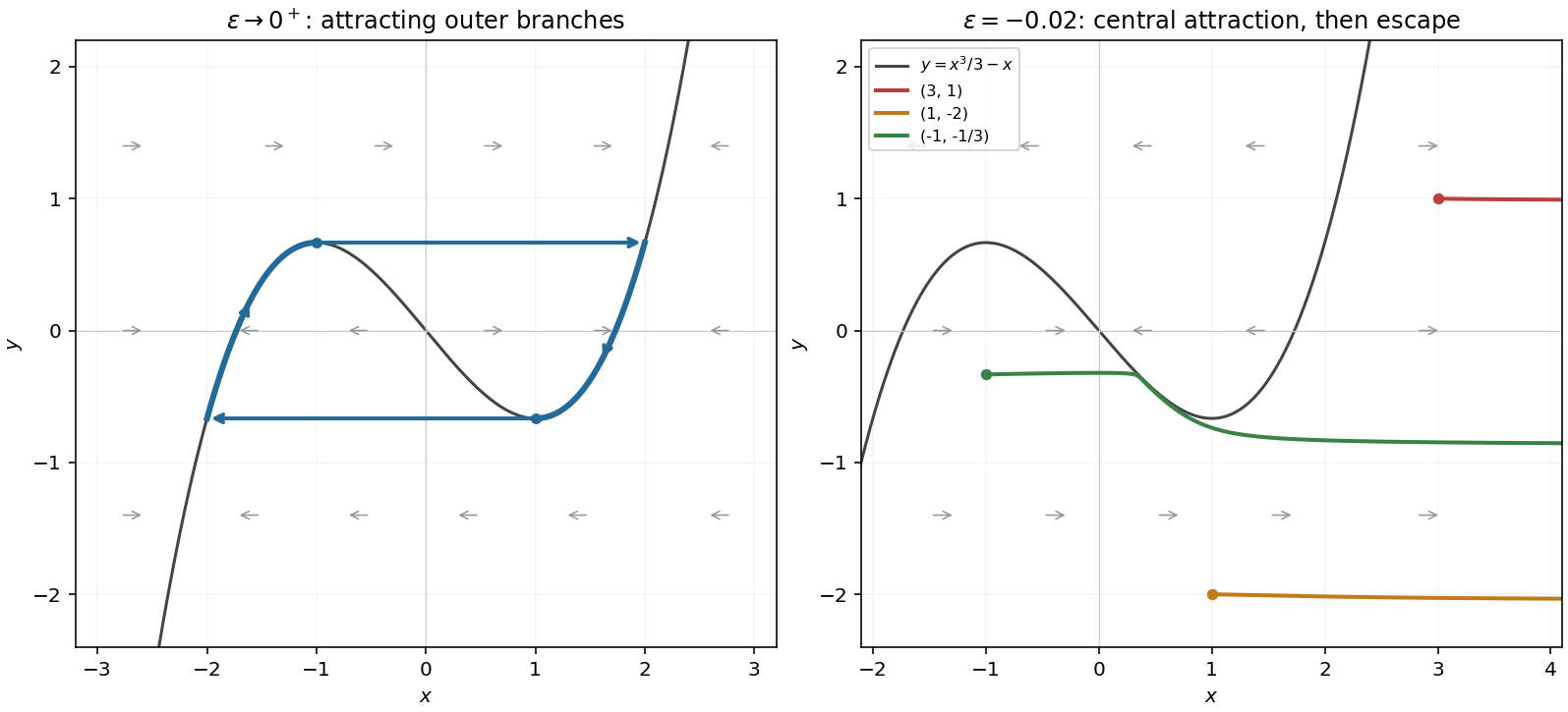
For negative $ϵ$ the fast arrows reverse: the outer branches become repelling and the middle branch attracting. On the middle branch the slow equation is $\dot{x}=x/(1-x^2)$, so the slow motion goes away from the saddle equilibrium at zero towards a fold.

At $(3,1)$, $F=3-9+1=-5$, so $\dot{x}>0$: the trajectory immediately escapes to the right. At $(1,-2)$, $F=1-1/3-2=-4/3$, so it also moves rapidly right and escapes. In each case the large-$x$ balance is $\dot{x}\sim x^3/(3|ϵ|)$, with $y$ decreasing; it is not a bounded relaxation cycle.

At $(-1,-1/3)$, $F=-1$, so the initial fast motion is rightward. At nearly fixed $y=-1/3$ it approaches the attracting middle root of $x-x^3/3=1/3$, approximately $x=0.347$. It then moves slowly down/right along the middle branch towards $(1,-2/3)$, leaves that fold to the right, and eventually escapes. These are the small-negative-$ϵ$ limiting descriptions; the fold locations and fast landing point receive small corrections. The right panel of the figure distinguishes this slow excursion from the two immediate escapes.

On the attracting right branch, $x>1$ and $\dot{y}=-x<0$, so the motion goes from $(2,2/3)$ towards the fold $(1,-2/3)$. At essentially fixed $y=-2/3$ it jumps to the other attracting root $x=-2$. The left branch then carries it to $(-1,2/3)$, where it jumps right to $x=2$. This gives the clockwise limiting relaxation oscillation shown in the preceding figure.

Along a slow branch $y=h(x)$, differentiation gives $(x^2-1)\dot{x}=-x$. The right-branch time isReflection symmetry gives the same time on the left. The fast jumps take a time tending to zero as $ϵ\to 0^{+}$, as do the fold-transition corrections at leading order. HenceThis is a leading asymptotic period, not an exact finite-$ϵ$ equality.

The nullcline is $\boxed{y=h(x)=x^3/3-x}$. Write $F=x-x^3/3+y$. Away from it at an order-one distance, $F$ is order one on the indicated finite phase-space scales. Thus $\dot{x}=O({ϵ}^{-1})$ while $\dot{y}=-x=O(1)$: the trajectory changes $x$ on the fast time in a singular perturbation $t/ϵ$, with only an $O(ϵ)$ change in $y$. Equivalently $dy/dx=-ϵx/F=O(ϵ)$, which explains the nearly horizontal motion.

For positive $ϵ$, $F_x=1-x^2$ makes the branches $|x|>1$ fast attracting and the middle branch $|x|<1$ fast repelling. The arrows point right where $y>h(x)$ and left where $y<h(x)$, carrying a generic off-nullcline point towards an attracting branch. The reduced description changes near a fold, where $F_x=0$; the rapid/slow distinction there needs a separate transition layer.

The left panel shows positive $ϵ$; the right panel shows negative $ϵ$, including the three specified starting points. Horizontal arrows indicate the leading fast motion.

Define the auxiliary variable $y=ϵ\dot{x}-x+x^3/3$. Differentiating gives $\dot{y}=ϵ\ddot{x}+(x^2-1)\dot{x}=-x$, while rearrangement gives $ϵ\dot{x}=x-x^3/3+y$. Conversely eliminating $y$ recovers the second-order equation, so this phase plane system is equivalent. At an equilibrium $\dot{y}=0$ forces $x=0$, and the first equation then forces $y=0$. Its Jacobian matrix isThus $ϵ{\lambda }^2-\lambda +1=0$. Expanding $\sqrt{1-4ϵ}=1-2ϵ-2{ϵ}^2-4{ϵ}^3+O({ϵ}^4)$ givesFor sufficiently small positive $ϵ$ both are positive: the equilibrium is an unstable node. For negative $ϵ$ the fast root is negative and the slow root positive, so it becomes a saddle equilibrium.

Try $\rho =t^{a}f(\eta )$, $\eta =x/t^b$. The boundary data force $a=3$ and $f(0)=1$. The time derivative scales as $t^{a-1}$, advection as $t^{2a-b}$ and the source as $t^{a+c}$. Balancing all three gives $c=-1$ and $b=a+1=4$. Substitution then yieldsFor the pointwise initial trace at any fixed $x>0$, the far-profile requirement is $f(\eta )=o({\eta }^{3/4})$ as $\eta \to \infty$ on any smooth branch extending that far; a compact-support continuation also meets it. Solving or selecting a shock continuation was not required. The time-dependent source is singular at $t=0$, so the similarity reduction is stated on $t>0$.

The nonzero kernel of $L$ rules out a unique solution for every value of $c$. By the Fredholm alternative, solvability requires orthogonality of the forcing to $\ker L^{\ast }=\mathrm{span}\{3a-5b\}$. Its pairing with $6a+cb$ isThus only $c=-4$ is compatible. In that case $6a-4b=2y_{-4}$ and a particular solution is $-y_{-4}/2$. All solutions areTherefore infinitely many solutions exist for $c=-4$, no solution exists for $c\ne -4$, and no parameter value gives a unique solution.

The adjoint also leaves $E$ invariant, with $L^{\ast }a=5a-15b$ and $L^{\ast }b=3a-9b$. By adjoint in weighted coordinates, its matrix in the same basis is $\left(\begin{array}{cc}5& 3\\ -15& -9\end{array}\right)$. Solving the two eigenvector equations givesThe basis $a,b$ is not orthonormal, so one must not simply transpose the previous numerical matrix without accounting for its Gram matrix. Directly transposing the integral kernel avoids that error.

Every eigenvector with eigenvalue different from one lies in $E=\mathrm{span}\{a,b\}$, because $(\lambda -1)y=Ky\in E$. The elementary overlaps are $⟨a,a⟩=1/2$, $⟨a,b⟩=1/3$, $⟨b,b⟩=1/4$. ThusIts characteristic polynomial is $\lambda (\lambda +4)$, so the finite-multiplicity eigenpairs areEach eigenspace has dimension one. On $E^{\perp }$, both integrals defining $K$ vanish, so $Ly=y$. Thus $\boxed{\lambda =1}$ is also an eigenvalue, of infinite multiplicity, and there are no others.

Write the integral part as $Ky=12b⟨a,y⟩-30a⟨b,y⟩$, where $a(x)=e^{-x}$ and $b(x)=e^{-2x}$. The kernel is real, so its adjoint transposes the two arguments. HenceThis follows by exchanging the two integrations in the $L^2(0,\infty )$ inner product; the exponential factors make the finite-rank operators bounded.

The integral equation says precisely $h=L^{-1}z$ with the homogeneous mixed endpoint conditions. Since the supplied $h$ satisfies those conditions, apply $L$ directly:No integration is required. The absence of a zero eigenvalue established in (b)–(c) also proves uniqueness of this recovered forcing.

Expand a forcing in the complete orthonormal basis ${\varphi }_n$. Since $L{\varphi }_n=-{\lambda }_n{\varphi }_n$, its inverse multiplies the $n$th coefficient by $-1/{\lambda }_n$. ConsequentlyThe negative sign follows from the eigenvalue convention $Ly=-\lambda y$. This kernel satisfies the mixed endpoint conditions in its first argument and $L_{x}g=\delta (x-t)$.

The difference of two solutions would satisfy $Ly=0$ with $y(0)=0$, $y^{\prime }(1)=0$. This would be a zero eigenvalue of the homogeneous problem, but part (b) shows there is none. Hence at most one solution exists. For continuous forcing the standard second-order existence construction also works: the free initial slope is fixed by an equation with coefficient $\cos 1\ne 0$. Thus for the stated regular boundary-value problem the solution is unique even with nonzero endpoint data.

The equation is $y^{\prime \prime }+(1+\lambda )y=0$. If $1+\lambda \le 0$, the linear or hyperbolic branches cannot meet both homogeneous endpoint conditions nontrivially. Otherwise $y=C\sin (kx)$, $k=\sqrt{1+\lambda }$, and $y^{\prime }(1)=Ck\cos k=0$ gives $k_n=(n+1/2)\pi$. ThereforeThe factor $\sqrt{2}$ makes the eigenfunctions unit normalized. All the eigenvalues are positive, in particular none is zero.

Let $L=D^2+1$ on the mixed endpoint domain $y(0)=0$, $y^{\prime }(1)=0$ in $L^2(0,1)$. Integration by parts gives the boundary formAt zero, $y^{\prime }(0)$ is free, forcing $z(0)=0$; at one, $y(1)$ is free, forcing $z^{\prime }(1)=0$. Therefore the formal adjoint expression and full adjoint endpoint conditions coincide with the original ones:With the usual second-order operator domain this is a self-adjoint problem. The consequences for its eigenvalues and eigenfunctions follow below.