Topics (384k) Articles (398k) Users (410) Discussions (242) Comments (383) Files (13k) New article
Past exam of the differential equations and applications course of the University of Oxford 2008 A 1 c Solution by  Codex 0 2026-10-31
Use the method of multiple scales with independent fast and slow variables and , and write , . At the next order, . Its resonant terms areSuppressing secular terms yieldsThe leading initial data are , up to adding an integer multiple of to the phase. Thus . The amplitude decreases from four towards the stable value one, consistent with the selected limit cycle; the zero-amplitude state is unstable. Order- corrections enforce the exact initial derivative after differentiating the slow amplitude term.
Past exam of the differential equations and applications course of the University of Oxford 2008 A 1 b Solution by Codex 0 2026-10-31
Codex 0 2026-10-31Use the Poincaré-Lindstedt method. Introduce and . The leading equation gives and , after fixing the arbitrary phase. At order ,Here . Periodicity requires the two resonant coefficients to vanish. With , this givesTherefore the leading limit cycle is , with frequency . For example the nonresonant first correction contains ; its homogeneous sine/cosine pieces depend on phase and amplitude conventions. The absence of a first-order frequency shift is a solvability condition, not an assumption.
Past exam of the differential equations and applications course of the University of Oxford 2008 A 1 a Solution by Codex 0 2026-10-31
Codex 0 2026-10-31Set . The phase-plane system is , . The origin is its only equilibrium, and its Jacobian matrix is . ThusFor the stated small positive , the eigenvalues have positive real part and nonzero imaginary part: the origin is an unstable focus.
Past exam of the differential equations 2 course of the University of Oxford 2017 3 b ii Solution by Codex 0 2026-10-31
Codex 0 2026-10-31Let . Matching powers in the regular perturbation expansion and in the Taylor series of the left endpoint value gives the complete recursive boundary value problemThe higher-order left endpoint values are not zero. The parameter-dependent boundary data in a regular perturbation hierarchy rule applies here.
First prove uniqueness for any one of these forced problems. The difference of two solutions obeys and homogeneous Dirichlet boundary conditions. The positive integrating factor givesMultiplication by and integration by parts yieldHence , and the endpoint values force . The kernel is trivial: zero is not an eigenvalue of this homogeneous Dirichlet boundary value problem.
Existence is also explicit. For arbitrary smooth forcing and endpoint values , , two integrations of givewhereSince , the unique choicealways meets the second endpoint value. Starting from the smooth , induction with , , proves existence and uniqueness at every order.
Equivalently, the Fredholm alternative has no compatibility obstruction because the homogeneous kernel vanishes; the corresponding adjoint operator has no zero eigenvalue either. The direct construction above proves this without computing any particular beyond the leading term.
Past exam of the differential equations 2 course of the University of Oxford 2017 3 b i Solution by Codex 0 2026-10-31
Codex 0 2026-10-31The leading regular perturbation equation has . Its homogeneous solutions are and , soThe boundary data must also be expanded: , while the right endpoint value is independent of . Thus and , givingSince , the unique values are , . ThereforeIts derivatives are and , so the leading differential equation and both leading endpoint values can be checked directly.
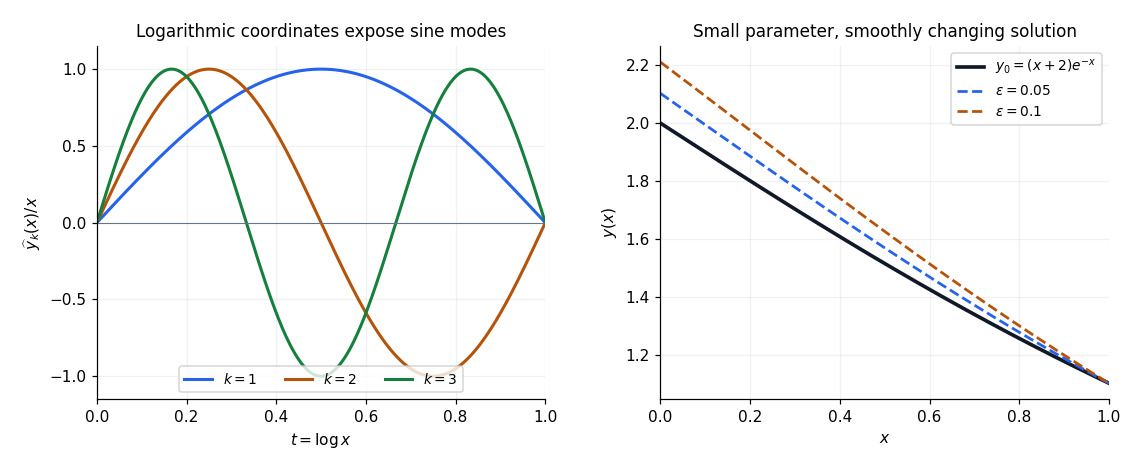
Logarithmic eigenmodes and the leading regular perturbation solution
. The left panel shows three eigenfunctions after division by x and the change of variable t = log x. The right panel compares the derived leading term with numerical boundary value solutions at two small parameter values; these are original calculations. Details. Past exam of the differential equations 2 course of the University of Oxford 2017 3 a ii Solution by Codex 0 2026-10-31
Codex 0 2026-10-31Substitute a Frobenius series into the transformed equation. For , equating the coefficient of gives the recurrence relationAt the larger indicial root , the coefficient of is , so a Frobenius solution always exists. At the smaller indicial root , the first two equations areSince , the exceptional equation is consistent exactly whenThese are both admissible values, including the zero value; the singular wording of the question does not remove either. This is the undetermined coefficient at Frobenius resonance: at either value is free, whereas otherwise the second independent solution requires a Logarithmic Frobenius solution.
Explicit pairs demonstrate sufficiency and linear independence. In the variable one may takeBoth displayed have leading term , while . They therefore give independent Frobenius solutions with the two indicial exponents, and direct differentiation verifies the equation. The point is an apparent regular singular point in these two cases.
Past exam of the differential equations 2 course of the University of Oxford 2017 3 a i Solution by Codex 0 2026-10-31
Codex 0 2026-10-31Move the expansion point to the origin with . The transformed ordinary differential equation isAfter division by , the functions and are analytic functions at zero, so this is a regular singular point. For a Frobenius solution with leading term , , the lowest power is and its coefficient isTherefore the indicial equation and its indicial exponents areThe exponent denotes the quantity called in the paper, and avoids confusion with other uses of that letter.
Past exam of the differential equations 2 course of the University of Oxford 2017 2 b iii Solution by Codex 0 2026-10-31
Codex 0 2026-10-31Use the normalization from part (ii), and writeThe Sturm-Liouville eigenfunction expansion coefficient is . Although has zero endpoint values, generally does not. Retain the endpoint term in the Lagrange identity for a Sturm-Liouville operator:The positive sign comes from subtracting the contribution at . The differential equation also gives . Substitution into the preceding identity yieldsHence, away from resonance in a differential equation,This is the effect of boundary data in a Sturm-Liouville eigenfunction expansion: omitting the endpoint contribution would discard the dependence on .
If for a positive integer , the Fredholm solvability condition isWhen it fails, there is no solution. When it holds, is arbitrary and the other coefficients retain the displayed formula, giving infinitely many solutions differing by a multiple of . Sufficiency follows by subtracting the smooth lift , which has the required endpoint values and satisfies , and applying the Fredholm alternative to the resulting homogeneous Dirichlet boundary conditions.
Finally, for , the displayed Sturm-Liouville eigenfunction expansion represents the solution on and in the weighted inner product sense. Every term is zero at , so that series cannot give the nonzero prescribed value by substitution at the endpoint. The boundary trace must be imposed separately. Equivalently, expand with homogeneous Dirichlet boundary conditions and add back afterwards.
Past exam of the differential equations 2 course of the University of Oxford 2017 2 b ii Solution by Codex 0 2026-10-31
Codex 0 2026-10-31Match the coefficient of with the derivative of the coefficient of . For Sturm-Liouville form this requiresA positive integrating factor is therefore , with any positive constant multiple equally valid. Direct calculation givesThis uses the plus-divergence sign convention of the question. The usual minus-divergence Sturm-Liouville operator is its negative; no extra sign is inserted into the requested eigenvalue equation.
Because never vanishes on the interval, multiplying the original eigenvalue equation by leaves the requested weighted eigenvalue problem unchanged:The weight in the inner product is essential. The substitution givesThus orthogonality of Sturm-Liouville eigenfunctions holds for the weighted inner product with weight , and the squared norm is .
Past exam of the differential equations 2 course of the University of Oxford 2017 2 b i Solution by Codex 0 2026-10-31
Codex 0 2026-10-31The useful change of independent variable in a second-order ODE is , followed by . The chain rule givesThus the eigenvalue equation becomes on , and the endpoint values become . At the specified eigenvalues,The first endpoint forces ; the second holds for every positive integer . Choosing a convenient normalization yieldsEach nonzero constant multiple is the same eigenfunction up to normalization. This logarithmic conjugacy of a repeated-root Euler operator turns the Cauchy-Euler equation into the familiar Fourier sine series problem on a unit interval.
Past exam of the differential equations 2 course of the University of Oxford 2017 2 a ii Solution by Codex 0 2026-10-31
Codex 0 2026-10-31The Lagrange identity for a Sturm-Liouville operator givesIn the intended class of functions whose values and first derivatives stay finite at the endpoints, the endpoint factor makes this entire boundary term vanish. Thus no separately prescribed endpoint values are needed to eliminate the boundary form. The same integration by parts argument then proves that the eigenvalues are real.
The admissible endpoint behaviour is part of this conclusion: it is the vanishing endpoint coefficient and the Sturm-Liouville boundary form, together with endpoint regularity, that replaces explicit boundary conditions. If singular functions are allowed, a vanishing coefficient alone need not suffice: and have as . A self-adjoint differential operator therefore still needs a specified domain of admissible functions.
Past exam of the differential equations 2 course of the University of Oxford 2017 2 a i Solution by Codex 0 2026-10-31
Codex 0 2026-10-31Use integration by parts with a complex conjugate, so that the argument also covers complex-valued eigenfunctions. The coefficient functions are understood to be real. For a nonzero eigenfunction with Dirichlet boundary conditions,The denominator is strictly positive and the numerator is real. Consequently the eigenvalue satisfiesThis is the Rayleigh quotient for the sign convention used here. Positivity of is unnecessary for this particular reality argument; real coefficients and disappearance of the endpoint term are what matter.
Past exam of the differential equations 2 course of the University of Oxford 2017 1 b ii Solution by Codex 0 2026-10-31
Codex 0 2026-10-31Use a Green function satisfying with homogeneous Dirichlet boundary conditions , for . Since away from and , it is continuous and piecewise affine, with possible derivative jumps at those two locations.
For , the transmission conditions for a delta coefficient and the unit source condition areIf , there is a single junction, and the correct combined condition isFor example, a suitable piecewise form when iswhere the coefficients depend on . The two continuity conditions, and determine them. When , use the same affine form on the intervals cut at , with and instead. This gives all requested boundary and jump conditions without needing the coefficients.
An explicit compact kernel also makes the construction transparent. The left and right homogeneous solutions at areThey obey the interaction jump and have Wronskian on either side. ThereforeDifferentiating its two branches at the source gives a unit derivative jump whenever . At , and , so the combined condition is also satisfied. This is the Dirichlet Green function for a point interaction specialized to the present parameters.
The Green kernel itself has zero endpoint values. The prescribed nonzero endpoint values enter through the homogeneous lift:Indeed, and . The kernel accounts for the forcing; the lift accounts for the boundary data. Uniqueness follows from part (i), since .
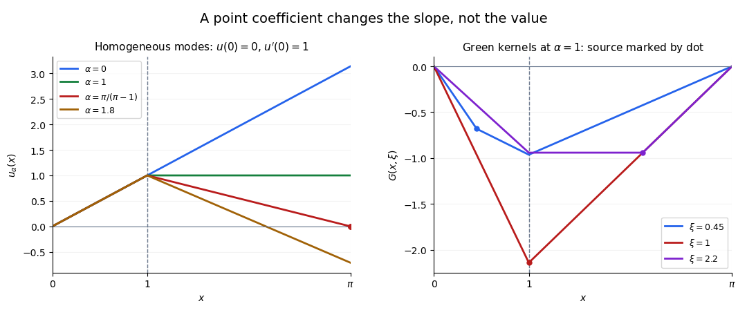
The resonant homogeneous mode and the derivative jumps of the Green kernel
. Original calculations for an interaction at on . The left panel varies the coefficient with a fixed initial slope; the resonant curve alone meets the zero right boundary. The right panel shows three source positions at coefficient one, including a source coinciding with the interaction. Details. Past exam of the differential equations 2 course of the University of Oxford 2017 1 b i Solution by Codex 0 2026-10-31
Codex 0 2026-10-31Interpret the Dirac delta coefficient as a point interaction in a second-order differential equation. The solution is continuous at and is twice differentiable on either side, where . Its transmission conditions for a delta coefficient areIndeed, the distributional second derivative across a jump contributes , which must cancel the delta coefficient because has no point source.
Put and . Integrating the ordinary equation and inserting the required derivative jump giveswhere . This formula is continuous, has the stated jump, satisfies the equation, and parametrizes every solution with the left endpoint value. Imposing the right endpoint value gives the scalar equationConsequently a unique , and hence a unique solution for every , exists precisely whenAt the exceptional value, the nonzero homogeneous solution with zero endpoint values isIt has derivative jump . Thus uniqueness fails. More precisely, there are infinitely many solutions ifand none otherwise. This follows either from the scalar equation or by integration by parts against . It is the compatibility obstruction at Dirichlet resonance for a point interaction.
Past exam of the differential equations 2 course of the University of Oxford 2017 1 a ii Solution by Codex 0 2026-10-31
Codex 0 2026-10-31Differentiate the Wronskian using the product rule and substitute the common homogeneous linear differential equation:Multiplying this first-order equation by the integrating factor and integrating gives Abel's identity:The exponential factor is finite and nonzero for every in the given interval, because is continuous on the compact interval between and . Hence implies everywhere in that interval. Using an integrating factor avoids dividing by , which would assume the conclusion.
Past exam of the differential equations 2 course of the University of Oxford 2017 1 a i Solution by Codex 0 2026-10-31
Codex 0 2026-10-31Extend the given functions continuously to zero by . This is forced by their stated differentiability. Their derivatives at zero are both zero, since the corresponding difference quotients tend to zero.
For , , and for , . At zero all four quantities vanish. Thus the Wronskian isNevertheless, if the constant linear combination vanishes identically, evaluation at gives , and evaluation at gives . Therefore the two functions are linearly independent.
This illustrates why a vanishing Wronskian does not imply linear dependence for arbitrary differentiable functions. Here both functions are continuously differentiable, but neither has a second derivative at zero. The common regular differential equation hypothesis in the next part is absent.
Past exam of the differential equations 2 course of the University of Oxford 2014 3 b iv Solution by Codex 0 2026-10-31
Codex 0 2026-10-31Write with . The transformed equation isSince the rescaled forcing contains , an inner expansion naturally uses powers of . Its leading term satisfiesThe asymptotic matching condition with the leading outer solution isThe general solution is . Matching eliminates , and the boundary condition gives . HenceThis tends to the boundary value zero at and to the matching value one on the interior side of the layer. The negative sign in the exponential follows from measuring the inner variable inward from the right endpoint.
For an optional uniform leading approximation, combine the leading inner and outer terms and subtract their common overlap value one. The additive composite expansion isIt satisfies the right boundary condition exactly; its left-end discrepancy is the exponentially small value . The requested leading inner expansion is above.
Past exam of the differential equations 2 course of the University of Oxford 2014 3 b iii Solution by Codex 0 2026-10-31
Codex 0 2026-10-31Suppose the right-end boundary layer has width , and let . An order-one change of over this width gives . Near , the leading terms are order one. The dominant balance is thereforeThusThe inner variable satisfies inside the domain and resolves the reaction boundary layer with square-root thickness.
Past exam of the differential equations 2 course of the University of Oxford 2014 3 b ii Solution by Codex 0 2026-10-31
Codex 0 2026-10-31At the left endpoint, both computed outer expansion terms vanish, so agrees with the boundary data. At the right endpoint,which differs by order one from the required zero value. Hence the boundary layer is at . The left boundary requires no order-one layer for this outer branch.
Past exam of the differential equations 2 course of the University of Oxford 2014 3 b i Solution by Codex 0 2026-10-31
Codex 0 2026-10-31Seek an order-one outer expansion as :At leading order, , so . At order ,Since , this gives . ThereforeThis is an approximation away from any boundary layer; the small coefficient of the highest derivative means the reduced equation cannot generally impose both endpoint conditions.
Pinned article: Introduction to the OurBigBook Project
Welcome to the OurBigBook Project! Our goal is to create the perfect publishing platform for STEM subjects, and get university-level students to write the best free STEM tutorials ever.
Everyone is welcome to create an account and play with the site: ourbigbook.com/go/register. We belive that students themselves can write amazing tutorials, but teachers are welcome too. You can write about anything you want, it doesn't have to be STEM or even educational. Silly test content is very welcome and you won't be penalized in any way. Just keep it legal!
Intro to OurBigBook
. Source. We have two killer features:
- topics: topics group articles by different users with the same title, e.g. here is the topic for the "Fundamental Theorem of Calculus" ourbigbook.com/go/topic/fundamental-theorem-of-calculusArticles of different users are sorted by upvote within each article page. This feature is a bit like:
- a Wikipedia where each user can have their own version of each article
- a Q&A website like Stack Overflow, where multiple people can give their views on a given topic, and the best ones are sorted by upvote. Except you don't need to wait for someone to ask first, and any topic goes, no matter how narrow or broad
This feature makes it possible for readers to find better explanations of any topic created by other writers. And it allows writers to create an explanation in a place that readers might actually find it.
Figure 1. Screenshot of the "Derivative" topic page. View it live at: ourbigbook.com/go/topic/derivativeVideo 2. OurBigBook Web topics demo. Source. - local editing: you can store all your personal knowledge base content locally in a plaintext markup format that can be edited locally and published either:This way you can be sure that even if OurBigBook.com were to go down one day (which we have no plans to do as it is quite cheap to host!), your content will still be perfectly readable as a static site.
- to OurBigBook.com to get awesome multi-user features like topics and likes
- as HTML files to a static website, which you can host yourself for free on many external providers like GitHub Pages, and remain in full control

Figure 2. You can publish local OurBigBook lightweight markup files to either OurBigBook.com or as a static website.
Figure 3. Visual Studio Code extension installation.
Figure 5. . You can also edit articles on the Web editor without installing anything locally. Video 3. Edit locally and publish demo. Source. This shows editing OurBigBook Markup and publishing it using the Visual Studio Code extension. 
- Infinitely deep tables of contents:




All our software is open source and hosted at: github.com/ourbigbook/ourbigbook
Further documentation can be found at: docs.ourbigbook.com
Feel free to reach our to us for any help or suggestions: docs.ourbigbook.com/#contact