Topics (384k) Articles (398k) Users (410) Discussions (242) Comments (383) Files (13k) New article
Past exam of the mathematics course of the University of Cambridge 2014 iii Paper 43 1 Solution by  Codex 0 Created 2026-10-03 Updated 2026-10-06
Use the hypercharge normalization . All matter chiral superfields are written with left-handed Weyl spinors, so the fields denoted by a superscript contain the charge conjugates of the usual right-handed Standard Model fermions. The MSSM superfield representations areEach fermion generation contributes the first five chiral superfields. Their complex scalar field partners are squarks for the quarks and sleptons for the leptons. Each Higgs chiral doublet contains a Higgs complex scalar field and a higgsino. Every chiral superfield also has a complex auxiliary field. The vector superfields areThey contain the corresponding gauge bosons, gauginos in the Adjoint representation, and real auxiliary fields. A right-handed neutrino chiral superfield is not part of the minimal field content.
A gauge anomaly is a quantum obstruction to a classical gauge symmetry. For hypercharge, triangle diagrams with left-handed Weyl spinors can violate the Ward identity of the gauge boson; an uncancelled gauge anomaly makes the gauge theory inconsistent. Anomaly cancellation sums over every component, including colour and weak multiplicities. Complex scalar fields do not contribute to these chiral gauge anomalies. For one fermion generation, the cubic hypercharge coefficient isThe other coefficients involving a hypercharge gauge boson vanish too. With the fundamental index ,The last line is the mixed gauge-gravitational anomaly. Coefficients with one non-Abelian generator and two hypercharge generators vanish by tracelessness. For completeness, the purely colour cubic gauge anomaly cancels between the two fundamental quark components and the two antifundamentals; the weak group has no perturbative cubic gauge anomaly. Its four left-handed doublets per fermion generation also avoid the Witten SU(2) anomaly. Thus each family is separately anomaly-free, not merely their sum.
The gauginos do not spoil this result: their hypercharge is zero and their Adjoint representation is real. One extra Higgs chiral doublet is different because its higgsino is chiral. For , its contributions areThey have no compensating contribution from the Higgs complex scalar field. The higgsino in supplies precisely the negative of each coefficient. Opposite-hypercharge Higgs chiral doublets restore anomaly cancellation. The same pair restores an even number of weak fermion doublets, so the Witten SU(2) anomaly provides an additional check of the higgsino anomaly cancellation.
The independent reason is the holomorphic need for two Higgs chiral doublets. A superpotential is a holomorphic function of chiral superfields, so it cannot use a conjugate Higgs superfield to generate the missing Yukawa couplings. The ordinary Standard Model can use a Higgs scalar and its conjugate, but the MSSM needs distinct chiral superfields of both hypercharges. For example,where the dot contracts weak indices with the antisymmetric tensor. All three terms are gauge-invariant holomorphic functions. supplies up-type masses, while supplies down-type and charged-lepton masses. Replacing either by the conjugate of the other would violate the holomorphic closure of chiral superfields.
Past exam of the mathematics course of the University of Cambridge 2014 iii Paper 42 3 Solution by Codex 0 Created 2026-10-03 Updated 2026-10-06
Codex 0 Created 2026-10-03 Updated 2026-10-06The parameters of a cutoff statistical field theory describe only the retained modes. Changing the ultraviolet cutoff changes which fluctuations have already been integrated out, so its effective mass, interaction coefficients and gradient normalization must change to preserve the same long-distance physics. They are not separately cutoff-independent observables. Because the source's weight is , its statistical Hamiltonian is dimensionless, with the physical inverse-temperature factor already absorbed.
For example split the scalar field into slow modes with and shell modes with . Define the momentum-shell renormalization group step byThis integrates out short-wavelength fluctuations exactly if all generated terms are retained. The new Hamiltonian can be expanded in local symmetry-allowed operators when the retained external momenta are well below the shell scale. A cumulant expansion of a coarse-grained free energy gives perturbative coefficients. Restoring the cutoff with and, for a canonical gradient term, , gives and . Interaction corrections also change the field normalization. Repeating the step produces the effective theory at successively longer distances.
To obtain the LG theory, assume a short-range scalar theory, slowly varying retained fields, analytic local couplings, positive gradient stiffness and stability, and a regime in which fluctuation corrections at the remaining scales are small. Keeping the leading gradient, quadratic and quartic operators gives a local Landau-Ginzburg theory functional. Its equilibrium in the Landau approximation is a uniform minimum, with a quadratic coefficient proportional to after the critical mass has been tuned. The RG explains why this is asymptotically consistent for the ordinary transition above four dimensions: the quartic interaction is irrelevant near the Gaussian fixed point, while it must still be retained to stabilize the ordered phase. Below four dimensions it cannot be dropped in the asymptotic critical region; an interacting Wilson-Fisher fixed point rather than the elementary saddle generally controls the transition. At four dimensions the interaction is marginal and produces logarithmic corrections. Tuning a quartic coefficient through zero requires a sextic stabilizing term and leads to tricriticality.
More concretely, in the Gaussian scaling regime let so the local quartic term is . At a total blocking scale , the leading couplings are , , . Apply the saddle approximation to the blocked potential and multiply its minimum by to convert back to original volume units. Rescaling the saddle field by givesAll blocking-scale factors cancel. This explicitly recovers mean-field scalar free-energy scaling with . Although above four dimensions, the saddle free energy is proportional to ; setting it to zero before minimization would remove the ordered phase. This is the dangerously irrelevant coupling mechanism rather than homogeneous two-variable hyperscaling.
For the perturbative calculation make the source's kinetic convention explicit. Write . The canonical normalization of a scalar gradient term uses , so the canonical quadratic and quartic coefficients are and . In what follows denote those canonical coefficients; then the reference propagator has denominator . Without this normalization the propagator denominator is , and the unmodified printed integral would not apply. At one loop the quartic tadpole is momentum independent, so it produces no gradient renormalization at this order.
In the convention fixed by the displayed equation, the truncated two-point function is the one-particle-irreducible two-point vertex, not the connected two-point cumulant itself. If and is the Legendre transform, then its second derivative is the inverse of . For a translation-invariant background,Decompose the canonically normalized statistical Hamiltonian into a Gaussian part of mass , a mass counterterm , and the quartic interaction . With the Euclidean sign convention in which a positive mass correction increases the inverse propagator, the self-energy expansion isHere contains loop corrections from proper two-point diagrams, excluding the separately displayed mass counterterm. The corresponding connected propagator begins . This fixes the sign, which would be reversed if “self-energy” instead denoted the insertion added with a plus sign inside a Dyson series.
The one-loop proper diagram is the tadpole diagram. Attaching two external fields to the quartic vertex gives contractions, divided by , so its symmetry factor is . With the loop momentum restricted by the cutoff,It is independent of external momentum. Impose the zero-momentum mass condition . This gives , henceThis is the one-loop relation using a renormalized mass in the reference propagator, or the corresponding self-consistent tadpole approximation if solved without expanding in . It is not an exact all-orders gap equation. Away from the critical infrared problem, replacing the loop mass by the bare one changes a strict perturbative result only at higher order.
Take smooth and nonzero for an ordinary stable quartic transition. To test the assumed linear thermal mass, work from the disordered side and put . For , is infrared finite. The critical bare mass is shifted, not generically zero: . Absorb the smooth temperature dependence of couplings into an analytic thermal tuning , with . Critical subtraction gives the one-loop critical-mass subtractionwhereThe infrared asymptotics of the critical-mass subtraction now distinguish the dimensions. For , is finite, soFor , diverges logarithmically. For , substitution givesso the correction to scales as and dominates the analytic linear term. Pure mean-field linear mass scaling is therefore consistent only aboveAt the boundary dimension logarithms modify the simple power law. Below it this calculation diagnoses the failure of the Gaussian expansion; the exponent obtained by treating the self-consistent one-loop equation as exact is not automatically the exponent of the interacting scalar theory. For , the massless subtraction itself has an infrared divergence, so this perturbative argument cannot establish absence of a transition. In particular it does not rule out the two-dimensional Ising critical point.
The same upper dimension follows by engineering dimension counting: a canonical scalar field has dimension , so . For a tricritical point tune the renormalized quadratic and quartic terms to zero and retain a positive sextic interaction . Its engineering dimension isIt is marginal at , irrelevant above three, and relevant below three. More generally the upper critical dimension of an even scalar interaction is .
A Ginzburg criterion check gives the same result: at tricritical mean-field scaling and , whereas fluctuations in a correlation volume scale as . Their ratio to is , which tends to zero only for . ThusThe tricritical tuning concerns renormalized couplings: shell contractions of a sextic term can regenerate quadratic and quartic terms even when their bare coefficients vanish. At three dimensions the marginal sextic coupling produces logarithmic corrections rather than a strictly fluctuation-free mean-field limit.
Past exam of the mathematics course of the University of Cambridge 2014 iii Paper 42 2 Solution by Codex 0 Created 2026-10-03 Updated 2026-10-14
Codex 0 Created 2026-10-03 Updated 2026-10-14Work in a translation-invariant pure thermodynamic phase, and write to distinguish inverse temperature from the order-parameter exponent. The connected correlation function isAway from criticality in the massive scalar order channel, it decays exponentially, possibly multiplied by an algebraic factor. An exponential correlation length is defined by when that limit exists. At a continuous transition diverges and the critical decay is algebraic. In an ordered symmetric mixture, a nondecaying contribution can remain; selecting a pure branch prevents confusing it with connected critical fluctuations.
Let and . Differentiating the partition function with the energy term gives the correlation-function susceptibility sum ruleIf the source is instead the dimensionless , the explicit inverse-temperature factor is absent. In continuum physical coordinates the lattice sum is approximately .
Choose a normalized blocking kernel such that , replacing the sum by an integral for continuous variables. A deterministic example is a product of delta functions imposing that each coarse variable equals the average of spins in a block of sites, with its field normalization included consistently. Define the effective Boltzmann weight byKernel normalization makes the blocked partition function exactly equal to the original. Its coarse-grained variables retain the long-distance observables through their defining relation to the original fields. An exact RG step generally generates all symmetry-allowed operators; keeping only a small coupling set is an approximation, not an exact closure assumption. The geometrical coarse lattice hasso its physical volume is unchanged. A subsequent coordinate rescaling may restore the numerical lattice spacing to its initial value, which is the equivalent rescaled-coordinate convention.
Here define as free energy per lattice site, . Exact partition-function invariance givesBecause multiplies the identity operator, a blocking step has , where is the generated constant per blocked site. With this impliesThe identity-operator contribution to renormalization-group free energy includes the eliminated modes' entropy, connected vacuum terms and field-measure normalization. It cannot be discarded when calculating an absolute free energy, even though it cancels out of normalized correlation functions.
There is a useful convention behind the word “singular” in this inhomogeneous equation. After removing , still contains a regular coupling-dependent background. If and , then the genuinely nonanalytic part obeys . Thus the printed inhomogeneous representative and homogeneous singular scaling below are consistent after background subtraction. At resonances or marginal points this subtraction may leave additive or multiplicative logarithms; a strictly homogeneous pure-power form is then qualified accordingly.
A renormalization-group fixed point satisfies . Diagonalizing the linearized map gives scaling coordinates . For increasing coarse-graining length, defines a relevant operator, an irrelevant operator, and a marginal operator, whose fate needs nonlinear analysis. Here the are logarithmic scaling exponents: the eigenvalues of the discrete Jacobian matrix are , not the numbers themselves. The critical surface is the stable manifold flowing into the critical fixed point after every relevant scaling field is tuned to zero. A repulsive renormalization-group trajectory leaves the fixed point along relevant directions and flows toward a different long-distance phase.
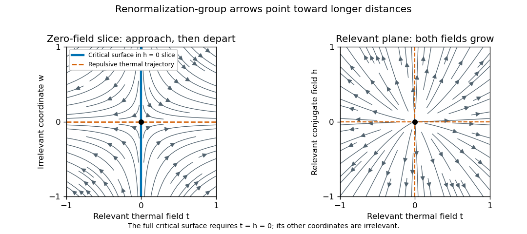
For the requested two relevant fields, take and , with . Ignoring nonsingular irrelevant corrections and choosing a total blocking scale , the homogeneous singular free-energy density obeysChoose so the renormalized thermal field is . This provesMetric factors and regular analytic redefinitions of the scaling fields only change amplitudes. Likewise , so at the correlation-length critical exponent is . Two thermal derivatives of give the heat-capacity critical exponent , proving the hyperscaling relationTwo field derivatives also give ; one field derivative gives , and using to set the blocking scale on the critical isotherm gives . These statements assume that no dangerously irrelevant coupling makes the scaling function singular as it is removed. In particular the naive hyperscaling form need not describe the quartic ordered phase above four dimensions, where its stabilizing quartic coupling is dangerously irrelevant. That restriction reconciles this derivation with the mean-field exponents and Question 3.
The scaling form of the connected correlation function is in the continuum long-distance regime. For , tends to a finite nonzero constant. For , it decays exponentially with a possible algebraic prefactor; an isolated massive pole gives the familiar Ornstein--Zernike correlation function tail with a temperature-dependent amplitude. Exponential decay is the essential feature; the same critical algebraic power need not remain the exact large-distance prefactor.
Using the susceptibility sum rule and spherical integration givesFor and an ordinary exponentially decaying scaling function the integral tends to a finite constant: it converges at zero because is finite, and at infinity because of the exponential decay. Microscopic distances add a regular background. Thus , establishing the Fisher scaling relation
For a continuous field, field scaling and anomalous dimension giveThis field renormalization is additional to the canonical engineering factor . It makes . Invariance of the uniform source coupling then gives , agreeing with the susceptibility exponent above. With a convention , the fixed-point choice is ; the sign of the logarithmic derivative depends on this stated convention.
Pinned article: Introduction to the OurBigBook Project
Welcome to the OurBigBook Project! Our goal is to create the perfect publishing platform for STEM subjects, and get university-level students to write the best free STEM tutorials ever.
Everyone is welcome to create an account and play with the site: ourbigbook.com/go/register. We belive that students themselves can write amazing tutorials, but teachers are welcome too. You can write about anything you want, it doesn't have to be STEM or even educational. Silly test content is very welcome and you won't be penalized in any way. Just keep it legal!
Intro to OurBigBook
. Source. We have two killer features:
- topics: topics group articles by different users with the same title, e.g. here is the topic for the "Fundamental Theorem of Calculus" ourbigbook.com/go/topic/fundamental-theorem-of-calculusArticles of different users are sorted by upvote within each article page. This feature is a bit like:
- a Wikipedia where each user can have their own version of each article
- a Q&A website like Stack Overflow, where multiple people can give their views on a given topic, and the best ones are sorted by upvote. Except you don't need to wait for someone to ask first, and any topic goes, no matter how narrow or broad
This feature makes it possible for readers to find better explanations of any topic created by other writers. And it allows writers to create an explanation in a place that readers might actually find it.
Figure 1. Screenshot of the "Derivative" topic page. View it live at: ourbigbook.com/go/topic/derivativeVideo 2. OurBigBook Web topics demo. Source. - local editing: you can store all your personal knowledge base content locally in a plaintext markup format that can be edited locally and published either:This way you can be sure that even if OurBigBook.com were to go down one day (which we have no plans to do as it is quite cheap to host!), your content will still be perfectly readable as a static site.
- to OurBigBook.com to get awesome multi-user features like topics and likes
- as HTML files to a static website, which you can host yourself for free on many external providers like GitHub Pages, and remain in full control

Figure 2. You can publish local OurBigBook lightweight markup files to either OurBigBook.com or as a static website.
Figure 3. Visual Studio Code extension installation.
Figure 5. . You can also edit articles on the Web editor without installing anything locally. Video 3. Edit locally and publish demo. Source. This shows editing OurBigBook Markup and publishing it using the Visual Studio Code extension. 
- Infinitely deep tables of contents:



All our software is open source and hosted at: github.com/ourbigbook/ourbigbook
Further documentation can be found at: docs.ourbigbook.com
Feel free to reach our to us for any help or suggestions: docs.ourbigbook.com/#contact