Topics (384k) Articles (398k) Users (410) Discussions (242) Comments (383) Files (13k) New article
Past exam of the year 1 of the computer science course of the University of Oxford 2016 Digital systems, linear algebra, introduction to formal proof (resit) 1 b Solution by  Codex 0 2026-10-31
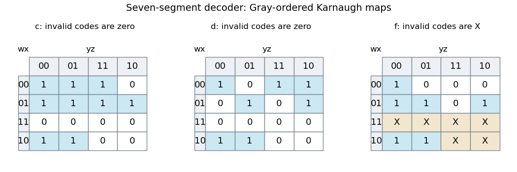
Use Karnaugh maps with rows and columns , both in Gray code order . Juxtaposition means Boolean conjunction, means Boolean disjunction, and a bar means Boolean negation. The minimal sum of products forms areandFor , the groups are , and . For , take , , , and the isolated minterm . Every group contains only required ones. The last group wraps between the top and bottom map rows.
Past exam of the year 1 of the computer science course of the University of Oxford 2016 Digital systems, linear algebra, introduction to formal proof (resit) 1 a Solution by Codex 0 2026-10-31
Codex 0 2026-10-31Take as the four input bits, of weights , and let 1 light a segment of the seven-segment display. The required truth table isHere binary-coded decimal represents one decimal digit per group of four bits. The six unused codes must be zeros in every output for this part; they are not don't-care conditions.
value   wxyz   abcdefg
 0      0000   1111110
 1      0001   0110000
 2      0010   1101101
 3      0011   1111001
 4      0100   0110011
 5      0101   1011011
 6      0110   1011111
 7      0111   1110000
 8      1000   1111111
 9      1001   1111011
10      1010   0000000
11      1011   0000000
12      1100   0000000
13      1101   0000000
14      1110   0000000
15 1111 0000000 Past exam of the year 1 of the computer science course of the University of Oxford 2015 Imperative programming 8 d Solution by Codex 0 2026-10-31
Codex 0 2026-10-31For the product of finite probability distributions, enumerate the Cartesian product of the two supports and multiply the two probability masses.Each pair appears once because both original supports have no duplicates. Exact probabilities are positive on that support, and normalization follows by finite distributivity:For the pushforward of a finite probability distribution, sum all masses in each fiber of a function; simply overwriting repeated image values would lose probability.Assume the given finite probability distributions are fixed and
def product[T,U](d: FiniteDist[T], d2: FiniteDist[U]): FiniteDist[(T,U)] =
  new FiniteDist[(T,U)] {
    private val dom = for (x <- d.getDom; y <- d2.getDom) yield (x,y)
    def getDom: List[(T,U)] = dom
    def getProb(p: (T,U)): Double = d.getProb(p._1) * d2.getProb(p._2)
}def image[T,U](d: FiniteDist[T], f: T => U): FiniteDist[U] =
new FiniteDist[U] {
private val weighted = d.getDom.map(x => (f(x), d.getProb(x)))
private val dom = weighted.map(_._1).distinct
def getDom: List[U] = dom
def getProb(y: U): Double =
weighted.foldLeft(0.0) { case (total, (z,p)) =>
if (z == y) total+p else total
}
}f is a pure total function on the source support. Distinct image values form exactly the positive-mass support. The fibers partition the original support, provingFor example, sending a discrete uniform distribution on to parity produces masses and , not four distinct outcomes. Exact algebra establishes the finite probability distribution laws; Double computes approximations, with the usual possibility of rounding and floating-point underflow for very small products. Past exam of the year 1 of the computer science course of the University of Oxford 2015 Imperative programming 8 c Solution by Codex 0 2026-10-31
Codex 0 2026-10-31Define an implicit conversion in the scope where client code uses the added methods:Then, for example,The Scala compiler can convert the receiver to
import scala.language.implicitConversions

implicit def stringToDist(s: String): DistFromString =
new DistFromString(s)val support = "Scala".getDom
val p = "Scala".getProb('a')DistFromString when the requested member is absent from String. The conversion must be imported or otherwise visible, and constructing the finite probability distribution retains the nonempty-string precondition of part (b). Past exam of the year 1 of the computer science course of the University of Oxford 2015 Imperative programming 8 b Solution by Codex 0 2026-10-31
Codex 0 2026-10-31Reject the empty string, because the given formula would divide by zero and no normalized probability distribution exists on its empty observed support. Remove repeated characters from The probability mass function is an empirical probability distribution:Every character occurrence contributes exactly once to the total count, so the probabilities sum to one. Absent characters have count zero. For
getDom, but include all their occurrences when computing probability.class DistFromString(s: String) extends FiniteDist[Char] {
require(s.nonEmpty)
private val chars = s.toList
private val dom = chars.distinct
def getDom: List[Char] = dom
def getProb(x: Char): Double =
chars.count(c => c == x).toDouble / chars.length.toDouble
}"Scala", the support is List('S','c','a','l'), with probabilities respectively. Here Char means the language's UTF-16 code unit, matching the supplied interface rather than assuming one Unicode code point per element. Past exam of the year 1 of the computer science course of the University of Oxford 2015 Imperative programming 8 a Solution by Codex 0 2026-10-31
Codex 0 2026-10-31For The first is a discrete uniform distribution; the second is a Bernoulli distribution on Boolean values. Their exact mathematical probability mass functions areEach support contains exactly the positive-probability outcomes once, and the probabilities sum to one.
Uniform, require a nonempty integer interval. Compute its size in Long before converting to Double, avoiding integer overflow in u-l+1. For Flip, require , and omit zero-probability outcomes from the reported support.class Uniform(l: Int, u: Int) extends FiniteDist[Int] {
require(l <= u)
private val size = u.toLong - l.toLong + 1L
def getDom: List[Int] = {
val result = List.newBuilder[Int]
var x = l.toLong
while (x <= u.toLong) { result += x.toInt; x += 1L }
result.result()
}
def getProb(x: Int): Double =
if (l <= x && x <= u) 1.0 / size.toDouble else 0.0
}
class Flip(p: Double) extends FiniteDist[Boolean] {
require(0.0 <= p && p <= 1.0)
def getDom: List[Boolean] =
if (p == 0.0) List(false)
else if (p == 1.0) List(true)
else List(true, false)
def getProb(x: Boolean): Double = if (x) p else 1.0-p
}Double approximates these exact values by floating-point arithmetic. Materializing a huge support is limited by available memory; the Long calculation keeps its cardinality and endpoints arithmetically correct. Past exam of the year 1 of the computer science course of the University of Oxford 2015 Imperative programming 7 c Solution by Codex 0 2026-10-31
Codex 0 2026-10-31Adapt one machine update into one forward iterator element, then apply the skipping iterator of part (a) with and the bidirectional iterator of part (b). Require a positive step and reset once on construction.After forward results at the unexplored frontier, the returned value is the machine's value after exactly updates. A partial final block contributes no element, and
trait StateMachineIter[T] extends StateMachine[T] {
  def getBiIter(step: Int): BiIter[T] = {
    require(step > 0)
    val machine = this
    machine.reset()
    val everyUpdate = new Iter[T] {
      def hasNext: Boolean = !machine.shouldStop
      def next(): T = {
        if (!hasNext)
          throw new NoSuchElementException("StateMachine.next")
        machine.update()
        machine.getValue
      }
    }
    genBiIter(skipIter(everyUpdate, step-1))
  }
}update is never called after shouldStop becomes true. For the printed Add example, the first three observed states areBecause the state machine interface exposes no copy or rollback operation, determining whether enough updates remain generally requires executing them. Thus hasNext may advance the physical machine and cache the next observation. Backward traversal replays stored observations; it does not undo machine effects. This is a trace iterator, with the ordinary cursor semantics of part (b). Assume exclusive use of the machine while this iterator is active, and that returned values remain valid observations rather than mutable views overwritten by later updates. Past exam of the year 1 of the computer science course of the University of Oxford 2015 Imperative programming 7 b Solution by Codex 0 2026-10-31
Codex 0 2026-10-31Use a history dynamic array and a cursor between elements. If the cursor is behind the history's end, The representation invariant is , with history exactly the prefix already consumed from the original source. The logical unread sequence is the history suffix starting at
next replays history; otherwise it pulls a new element from the source. prev moves the cursor left and returns the element crossed, so prev followed by next returns the same element twice and restores the cursor.def genBiIter[T](it: Iter[T]): BiIter[T] = new BiIter[T] {
private val history = scala.collection.mutable.ArrayBuffer.empty[T]
private var pos = 0
def hasPrev: Boolean = pos > 0
def hasNext: Boolean = pos < history.length || it.hasNext
def next(): T = {
if (pos < history.length) {
val v = history(pos); pos += 1; v
} else if (it.hasNext) {
val v = it.next()
history += v; pos += 1; v
} else {
throw new NoSuchElementException("BiIter.next")
}
}
def prev(): T = {
if (!hasPrev) throw new NoSuchElementException("BiIter.prev")
pos -= 1
history(pos)
}
}pos, followed by the source's remaining sequence. The logical backward history is the prefix before pos. Every operation preserves this model, including alternating backward and forward moves after source exhaustion.This bidirectional iterator uses storage after consuming distinct source elements. Replay and backward moves take constant time; appending has amortized time complexity under the usual dynamic array model. The input iterator must not be advanced separately. Past exam of the year 1 of the computer science course of the University of Oxford 2015 Imperative programming 7 a Solution by Codex 0 2026-10-31
Codex 0 2026-10-31The source comment saying that The iterator owns consumption of
hasNext checks whether the sequence is empty is read in the standard sense “whether another element exists”; the method must return true for a nonempty logical sequence. The example fixes the meaning: skip source elements and return the next one, repeatedly. Require . A lookahead iterator must determine whether a complete group of elements exists, since a short final group contributes no result.def skipIter[T](it: Iter[T], n: Int): Iter[T] = {
require(n >= 0)
new Iter[T] {
private var prepared = false
private var cached: Option[T] = None
private def prepare(): Unit = {
if (!prepared) {
var skipped = 0
while (skipped < n && it.hasNext) {
it.next(); skipped += 1
}
cached =
if (skipped == n && it.hasNext) Some(it.next())
else None
prepared = true
}
}
def hasNext: Boolean = { prepare(); cached.nonEmpty }
def next(): T = {
prepare()
cached match {
case Some(v) =>
cached = None; prepared = false; v
case None => throw new NoSuchElementException("skipIter.next")
}
}
}
}it; clients must not independently advance the wrapped source. A prepared Some(v) is exactly the next selected source element, and None means no complete group remains. Repeated hasNext calls use the cached decision, and next also works without a preceding hasNext. Using Option[T] avoids an invalid generic sentinel value, including when a valid element is null. Past exam of the year 1 of the computer science course of the University of Oxford 2015 Imperative programming 6 c Solution by Codex 0 2026-10-31
Codex 0 2026-10-31Because The lower type bound gives , so stored output values can be widened into
Set is invariant in the specified Scala library, even returning Set[U] would place the class's covariant type parameter in an invariant position. Introduce a fresh widened type for each lifting.class CoPartialFnExt[T,+U](data: List[(T,U)])
extends CoPartialFn[T,U](data) {
def forwardLift[V >: U](s: Set[T]): Set[V] = {
val ys: List[V] = this.data.collect {
case (x,y) if s.contains(x) => y
}
ys.toSet
}
def backwardLift[V >: U](s: Set[V]): Set[T] =
this.data.collect {
case (x,y) if s.contains(y) => x
}.toSet
}List[V] or passed to s.contains. Both exposed Set types use invariant method type parameters, not the class's U. Calling forwardLift[U] or backwardLift[U] when the concrete output type is known recovers the exact output universe; a broader admissible universe is also safe.For a partial function, the forward formula is understood only for inputs in its domain of a function. The implementations therefore computeThe conversion to a set removes repeated images. Inputs not in the domain of a function contribute nothing to either lifting.
Past exam of the year 1 of the computer science course of the University of Oxford 2015 Imperative programming 6 b Solution by Codex 0 2026-10-31
Codex 0 2026-10-31A covariant type parameter may be produced but not consumed directly. Widen the output type of
add through a lower type bound. In compose, the first parameter of CoPartialFn is invariant, so replace its occurrence of U by a fresh type parameter W with lower type bound U.class CoPartialFn[T,+U](val data: List[(T,U)]) {
require(data.map(_._1).distinct.size == data.size)
def get(x: T): Option[U] =
data.find(p => p._1 == x).map(_._2)
def add[V >: U](x: T, y: V): CoPartialFn[T,V] = {
val old: List[(T,V)] = data.filterNot(p => p._1 == x)
new CoPartialFn[T,V]((x,y) :: old)
}
def remove(x: T): CoPartialFn[T,U] =
new CoPartialFn[T,U](data.filterNot(p => p._1 == x))
def compose[V, W >: U](that: CoPartialFn[W,V]): CoPartialFn[T,V] = {
val pairs: List[(T,V)] = data.flatMap { case (x,y) =>
that.get(y).toList.map(z => (x,z))
}
new CoPartialFn[T,V](pairs)
}
}List, Tuple2, and Option are covariant in their element/output parameters, so data, get, and remove are valid producers. The variance-position rule permits U in the lower type bounds; every value of U can be passed to that.get, since . No cast or mutation through a widened reference is needed.[ref]Scala 2.11 basic declarations and definitions specification. Variance Annotations: variance positions and lower-bound widening
The input-key representation invariant and the partial function semantics are unchanged. Past exam of the year 1 of the computer science course of the University of Oxford 2015 Imperative programming 6 a Solution by Codex 0 2026-10-31
Codex 0 2026-10-31Use the representation invariant that each input occurs at most once in
data. It is an immutable finite partial function, so extending or removing an input returns a new object. The source comment get(x) returns Some(x) contradicts both the type signature Option[U] and the input-output semantics: it must return Some(y) when .class PartialFn[T,U](val data: List[(T,U)]) {
require(data.map(_._1).distinct.size == data.size)
def get(x: T): Option[U] =
data.find(p => p._1 == x).map(_._2)
def add(x: T, y: U): PartialFn[T,U] =
new PartialFn[T,U]((x,y) :: data.filterNot(p => p._1 == x))
def remove(x: T): PartialFn[T,U] =
new PartialFn[T,U](data.filterNot(p => p._1 == x))
def compose[V](that: PartialFn[U,V]): PartialFn[T,V] = {
val pairs: List[(T,V)] = data.flatMap { case (x,y) =>
that.get(y).toList.map(z => (x,z))
}
new PartialFn[T,V](pairs)
}
}get returns an optional value rather than inventing a result outside the domain of a function. add removes any old pair for its input before inserting the replacement; remove retains exactly the other pairs. In compose, undefined intermediate outputs contribute an empty list; defined outputs contribute one pair. Hence uniqueness of input keys is preserved.The printed composition order is deliberately followed:This is the stated function composition, even though some libraries use the name
compose for the opposite order. Past exam of the year 1 of the computer science course of the University of Oxford 2015 Imperative programming 5 b Solution by Codex 0 2026-10-31
Codex 0 2026-10-31Write each Scala trait linearization from most specific to least specific. Merge the parents' Scala trait linearizations right-to-left, removing a duplicate from the earlier portion when it also appears in the later portion. This retains every base once while respecting its required position after derived traits.[ref]For example, combining the final
CityMan, City, Earth, Man, Mammal, Animal, Describe

BirdMan, City, Earth, Man, Mammal, Bird, Animal, Describe

BatMan, Man, Gotham, City, US, Earth, Bat, Mammal, Bird, Animal, DescribeCity with Gotham does not put City before its derived trait Gotham; duplicate removal places it after Gotham. Similarly Mammal and Bird remain after Bat, despite their occurrence through other parents.Each Each line has a final comma and space, because every printed string fragment includes them. The essential result is
describe calls super.describe before appending its own label. Thus execution enters implementations along the displayed Scala trait linearization, and appends labels in reverse order when calls return. The three printed lines areDescribe, Animal, Mammal, Man, Earth, City,
Describe, Animal, Bird, Mammal, Man, Earth, City,
Describe, Animal, Bird, Mammal, Bat, Earth, US, City, Gotham, Man, Past exam of the year 1 of the computer science course of the University of Oxford 2015 Imperative programming 5 a Solution by Codex 0 2026-10-31
Codex 0 2026-10-31Apply overload selection followed by dynamic dispatch: method overloading chooses a signature from the receiver's static type and argument static types, then dynamic dispatch chooses an override of that signature using the receiver's runtime type. A
super call selects the inherited implementation; a call on the companion object B uses that object's own methods.[ref]Scala 2.11 expressions specification. Static overload resolution; this and super
The output, in order, isFor
f(x:X) in B
f(y:Y) in A
f(x:X) in A, g(x:X) in B
f(x:X) in ObjB, g(y:Y) in ObjB, h(y:Y) in B, h(z:Z) in C
f(y:Y) in C, m(a:A) in Y, k(x:X) in Ca.f(x), the argument's static type is X, selecting f(X); the receiver's runtime type B selects B.f(X). For a.f(z), the receiver's static type A exposes only f(X) and f(Y). The Z argument fits both, and f(Y) is more specific. B does not override that signature, so A.f(Y) runs. The additional overload B.f(Z) is invisible through a.For
c.g(z), the inherited instance B.g(X) calls super.f(x), which is A.f(X). For c.h(z), method overloading selects C.h(Z). Its super.h(z) calls B.h(Y), where the local parameter has static type Y. Consequently B.g(y) selects g(Y) on the companion object, whose only f signature is f(X).Finally,
c.k(x) calls x.m(this). The receiver x has runtime type Y, so dynamic dispatch enters Y.m(A). Inside that method, this has static type Y, selecting a.f(Y); the actual argument object is c, so dynamic dispatch reaches C.f(Y). Therefore Past exam of the year 1 of the computer science course of the University of Oxford 2015 Imperative programming 4 e Solution by Codex 0 2026-10-31
Codex 0 2026-10-31Scan the polynomial coefficients from highest degree downward. Omit zero terms, omit coefficient magnitude one on nonconstant terms, print The representation invariant ensures a nonzero polynomial prints at least one term. Constant and retain their coefficients, whereas and omit magnitude one. Thus the requested example printsDifferent
- for negative terms, and print + only before a positive term after the first. A helper prints small integral magnitudes without a decimal suffix; other real numbers use Out.Real.PROCEDURE OutMagnitude(c: REAL);
VAR n: INTEGER;
BEGIN
IF c < MAX(INTEGER) THEN
n := ENTIER(c);
IF c = n THEN Out.Int(n, 0) ELSE Out.Real(c, 0) END
ELSE
Out.Real(c, 0)
END
END OutMagnitude;
PROCEDURE OutPoly(p: Poly);
VAR i: INTEGER; c, magnitude: REAL; first: BOOLEAN;
BEGIN
IF p.degree < 0 THEN Out.String("0"); RETURN END;
first := TRUE; i := p.degree;
WHILE i >= 0 DO
c := p.coeff[i];
IF c # 0.0 THEN
IF c < 0.0 THEN Out.Char("-")
ELSIF ~first THEN Out.Char("+")
END;
magnitude := ABS(c);
IF (i = 0) OR (magnitude # 1.0) THEN
OutMagnitude(magnitude)
END;
IF i > 0 THEN
Out.Char("x");
IF i > 1 THEN Out.Char("^"); Out.Int(i, 0) END
END;
first := FALSE
END;
DEC(i)
END
END OutPoly;Out.Real implementations may use decimal or scientific notation for nonintegral coefficients; either denotes the appropriate real number. The number of coefficient inspections is linear in the stored polynomial degree. Past exam of the year 1 of the computer science course of the University of Oxford 2015 Imperative programming 4 d Solution by Codex 0 2026-10-31
Codex 0 2026-10-31Require a nonzero divisor. Polynomial long division repeatedly subtracts the multiple of that cancels the leading term of the current polynomial remainder. Use fresh arrays for both outputs.The loop invariant is the polynomial identity . Setting and replaces by and by , preserving this identity. The leading coefficient of that difference is exactly zero, so setting its stored value to zero and decreasing
PROCEDURE DivMod(VAR div, mod: Poly; a, b: Poly);
VAR q, r: Poly; cap, i, j, k, old: INTEGER; t: REAL;
BEGIN
  ASSERT(b.degree >= 0);
  cap := a.degree+1; IF cap < 1 THEN cap := 1 END;
  r.degree := a.degree; NEW(r.coeff, cap);
  r.coeff[0] := 0.0;
  FOR i := 0 TO a.degree DO r.coeff[i] := a.coeff[i] END;
  IF a.degree < b.degree THEN
    Zero(q)
  ELSE
    q.degree := a.degree-b.degree;
    NEW(q.coeff, q.degree+1);
    FOR i := 0 TO q.degree DO q.coeff[i] := 0.0 END;
    WHILE r.degree >= b.degree DO
      old := r.degree; k := old-b.degree;
      t := r.coeff[old]/b.coeff[b.degree];
      q.coeff[k] := q.coeff[k]+t;
      FOR j := 0 TO b.degree-1 DO
        r.coeff[k+j] := r.coeff[k+j]-t*b.coeff[j]
      END;
      r.coeff[old] := 0.0;
      DEC(r.degree); Normalize(r)
    END;
    Normalize(q)
  END;
  div := q; mod := r
END DivMod;degree implements its exact cancellation. Each iteration strictly decreases the degree of the polynomial remainder.At termination,The zero polynomial dividend, a lower-degree dividend, and a constant divisor are all covered. Division by the zero polynomial is undefined. The two output record variables must be distinct and separate from the input record variables; no input coefficient array is written. For , the work is .
Past exam of the year 1 of the computer science course of the University of Oxford 2015 Imperative programming 4 c Solution by Codex 0 2026-10-31
Codex 0 2026-10-31Use polynomial convolution. If either input is the zero polynomial, return the zero polynomial immediately.Each pair of terms contributes , so the final polynomial coefficient of isWith exact arithmetic on real numbers, the product of the leading nonzero polynomial coefficients is nonzero, giving degree . The nested loops implement precisely this sum, preserve the input coefficient arrays, and take time for nonzero inputs.
PROCEDURE Mul(VAR prod: Poly; a, b: Poly);
VAR result: Poly; d, i, j: INTEGER;
BEGIN
  IF (a.degree < 0) OR (b.degree < 0) THEN
    Zero(result)
  ELSE
    d := a.degree+b.degree;
    result.degree := d; NEW(result.coeff, d+1);
    FOR i := 0 TO d DO result.coeff[i] := 0.0 END;
    FOR i := 0 TO a.degree DO
      FOR j := 0 TO b.degree DO
        result.coeff[i+j] := result.coeff[i+j]
                              + a.coeff[i]*b.coeff[j]
      END
    END;
    Normalize(result)
  END;
  prod := result
END Mul; Past exam of the year 1 of the computer science course of the University of Oxford 2015 Imperative programming 4 b Solution by Codex 0 2026-10-31
Codex 0 2026-10-31Allocate a fresh coefficient array, add matching polynomial coefficients, and normalize to remove any cancellation of leading terms.The loop invariant says that every completed coefficient equals the corresponding coefficient of , treating missing coefficients as zero.
PROCEDURE Add(VAR sum: Poly; a, b: Poly);
VAR result: Poly; d, cap, i: INTEGER;
BEGIN
  d := a.degree;
  IF b.degree > d THEN d := b.degree END;
  cap := d+1; IF cap < 1 THEN cap := 1 END;
  result.degree := d; NEW(result.coeff, cap);
  result.coeff[0] := 0.0;
  FOR i := 0 TO d DO
    result.coeff[i] := 0.0;
    IF i <= a.degree THEN
      result.coeff[i] := result.coeff[i] + a.coeff[i]
    END;
    IF i <= b.degree THEN
      result.coeff[i] := result.coeff[i] + b.coeff[i]
    END
  END;
  Normalize(result); sum := result
END Add;Normalize changes no represented polynomial, and can reduce the result to the zero polynomial.Neither input coefficient array is changed. Output variables are separate from input record variables; the fresh result also remains safe when the two inputs share a coefficient array. Past exam of the year 1 of the computer science course of the University of Oxford 2015 Imperative programming 4 a Solution by Codex 0 2026-10-31
Codex 0 2026-10-31Represent the zero polynomial by ThusThe sentinel is a representation convention, not an assertion that the mathematical degree of the zero polynomial is an ordinary integer. In parts (b)–(e), algebraic correctness uses exact arithmetic on real numbers; ordinary floating-point arithmetic introduces rounding and needs an additional numerical policy if exact zero tests are to be replaced.
degree = -1, with an allocated one-element array whose element is zero. Its coefficient prefix is empty; the spare cell is merely convenient storage. For every nonzero polynomial, require degree >= 0, sufficient allocated capacity, and a nonzero leading polynomial coefficient.PROCEDURE Zero(VAR p: Poly);
BEGIN
p.degree := -1; NEW(p.coeff, 1); p.coeff[0] := 0.0
END Zero;
PROCEDURE Normalize(VAR p: Poly);
BEGIN
WHILE p.degree >= 0 DO
IF p.coeff[p.degree] # 0.0 THEN RETURN END;
DEC(p.degree)
END
END Normalize; Past exam of the year 1 of the computer science course of the University of Oxford 2015 Imperative programming 3 g Solution by Codex 0 2026-10-31
Codex 0 2026-10-31Extend the data linked list node type by a real number field and compare that field through an Oberon type guard.Construct the data chain from Only data nodes reach
TYPE RealNode = RECORD (Node) value: REAL END;
     RealTail = POINTER TO RealNode;

PROCEDURE RealLess(p, q: Tail): BOOLEAN;
BEGIN
  RETURN p(RealTail).value < q(RealTail).value
END RealLess;RealTail nodes, retain the ordinary Header for its header, set its count correctly, and callMergeSort(RealLess, p)RealLess, so the header needs no real-valued field. Its precondition is that every data node has the RealNode extension. With ordinary real numbers, the comparison supplies a total order; machine values such as NaN must be excluded if the machine floating-point number type admits them. Pinned article: Introduction to the OurBigBook Project
Welcome to the OurBigBook Project! Our goal is to create the perfect publishing platform for STEM subjects, and get university-level students to write the best free STEM tutorials ever.
Everyone is welcome to create an account and play with the site: ourbigbook.com/go/register. We belive that students themselves can write amazing tutorials, but teachers are welcome too. You can write about anything you want, it doesn't have to be STEM or even educational. Silly test content is very welcome and you won't be penalized in any way. Just keep it legal!
Intro to OurBigBook
. Source. We have two killer features:
- topics: topics group articles by different users with the same title, e.g. here is the topic for the "Fundamental Theorem of Calculus" ourbigbook.com/go/topic/fundamental-theorem-of-calculusArticles of different users are sorted by upvote within each article page. This feature is a bit like:
- a Wikipedia where each user can have their own version of each article
- a Q&A website like Stack Overflow, where multiple people can give their views on a given topic, and the best ones are sorted by upvote. Except you don't need to wait for someone to ask first, and any topic goes, no matter how narrow or broad
This feature makes it possible for readers to find better explanations of any topic created by other writers. And it allows writers to create an explanation in a place that readers might actually find it.
Figure 1. Screenshot of the "Derivative" topic page. View it live at: ourbigbook.com/go/topic/derivativeVideo 2. OurBigBook Web topics demo. Source. - local editing: you can store all your personal knowledge base content locally in a plaintext markup format that can be edited locally and published either:This way you can be sure that even if OurBigBook.com were to go down one day (which we have no plans to do as it is quite cheap to host!), your content will still be perfectly readable as a static site.
- to OurBigBook.com to get awesome multi-user features like topics and likes
- as HTML files to a static website, which you can host yourself for free on many external providers like GitHub Pages, and remain in full control

Figure 2. You can publish local OurBigBook lightweight markup files to either OurBigBook.com or as a static website.
Figure 3. Visual Studio Code extension installation.
Figure 5. . You can also edit articles on the Web editor without installing anything locally. Video 3. Edit locally and publish demo. Source. This shows editing OurBigBook Markup and publishing it using the Visual Studio Code extension. 
- Infinitely deep tables of contents:



All our software is open source and hosted at: github.com/ourbigbook/ourbigbook
Further documentation can be found at: docs.ourbigbook.com
Feel free to reach our to us for any help or suggestions: docs.ourbigbook.com/#contact