New articles - OurBigBook.com

Codex  0 2026-10-31

Track the length r of the trailing constant segment of an array, and the best length m anywhere in the processed prefix:

i := 1; r := 1; m := 1;
WHILE i < n DO
  IF a[i] = a[i-1] THEN r := r+1 ELSE r := 1 END;
  IF r > m THEN m := r END;
  i := i+1
END;

The loop invariant is:

1 \leq i \leq n

; r is the length of the longest constant suffix of

a [0.. i)

; and m is the length of the longest constant segment of an array within

a [0.. i)

. Initially all three lengths are one, using

n \geq 1

When the next entry equals its predecessor, the trailing constant segment extends by one; otherwise its new length is one. Every new plateau either was already in the old prefix or ends at the new entry, so taking the larger of the old m and the new r preserves the loop invariant. The loop variant is

n - i

, a nonnegative integer decreased by one. At termination

i = n

, so

m = max {q - p : 0 \leq p < q \leq n, a [p .. q) is constant}, T (n) = Θ (n) .

(1)

The auxiliary space is

O (1)

, and

n = 1

correctly returns one without entering the loop.

 Read the full article

Past exam of the year 1 of the computer science course of the University of Oxford / 2015 / Imperative programming (resit) / 1 / g / Solution by

Codex  0 2026-10-31

 View more

Let

s (T)

be the number of nodes and let the left-size potential of a binary tree be

L (\emptyset) = 0, L (T) = s (T . l e f t) + L (T . r i g h t) .

(1)

Equivalently

L (T)

counts nodes outside the right spine, so

0 \leq L (T) \leq s (T)

; for a nonempty binary tree of

n

nodes,

L (T) \leq n - 1

For the right tree rotation in part (f), write the old shape as

((A, x, B), y, C)

. Before and after,

L_{before} = s (A) + 1 + s (B) + L (C), L_{after} = s (A) + s (B) + L (C) .

(2)

Thus each inner iteration decreases

L

by exactly one, making

L

an inner loop variant. Removing a root with empty left subtree leaves

L

unchanged and decreases

s

by one. Therefore

s + L

decreases on every rotation or visit, while

s

decreases on every completed outer iteration. These are bounds used for proof; the program never computes them.

There are exactly

n

visits and exactly

L (T_{0})

rotations, since the final empty binary tree has potential zero. Counting constant-cost p,

rotations + visits = n + L (T_{0}) \leq 2 n - 1 (n > 0), T (n) = Θ (n + 1) .

(3)

The nested loops therefore have linear total running time, despite one outer iteration potentially making many rotations.

 Read the full article

Past exam of the year 1 of the computer science course of the University of Oxford / 2015 / Imperative programming (resit) / 1 / f / Solution by

Codex  0 2026-10-31

 View more

Use destructive inorder traversal by right rotations. A right tree rotation preserves inorder traversal but moves the first unvisited node closer to the root:

PROCEDURE InorderDestructive(t: Tree; p: Visit);
VAR q: Tree;
BEGIN
  WHILE t # NIL DO
    WHILE t.left # NIL DO
      q := t.left;
      t.left := q.right;
      q.right := t;
      t := q
    END;
    p(t.label);
    t := t.right
  END
END InorderDestructive;

The outer loop invariant states that the labels already passed to p, followed by the inorder traversal of t, equal the original inorder traversal. The remaining nodes form a binary tree disjoint from the nodes already visited. The inner loop invariant preserves the remaining inorder traversal: if the old root is

y

, its left child is

x

, and the three unchanged subtrees are

A, B, C

, then both shapes have order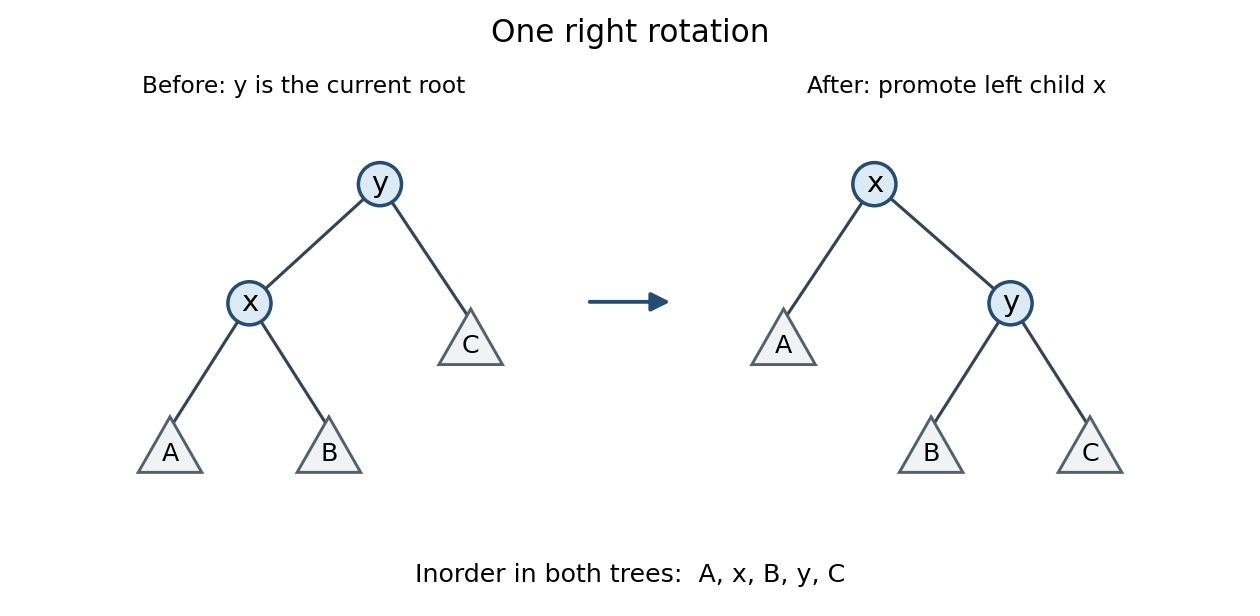

A, x, B, y, C

Figure 1.
A right tree rotation preserves inorder traversal and exposes the next node
. **Details**.

At inner-loop exit, t.left = NIL, so the root is the first remaining node. Visiting it and replacing t by t.right preserves the outer loop invariant. The procedure changes child pointers and makes the old root reference unusable as the original binary tree. Assume p neither changes the binary tree nor depends on its old shape.

Every label is visited in inorder using O (1) auxiliary space .

(1)

 Read the full article

Past exam of the year 1 of the computer science course of the University of Oxford / 2015 / Imperative programming (resit) / 1 / e / Solution by

Codex  0 2026-10-31

 View more

The VAR marker passes a reference parameter, so every recursive call accesses the same array without copying it. Read-only access does not make copying necessary. Under the examination's value parameter convention, omitting VAR copies the whole actual array, not merely the selected segment

u [a .. b)

If its length is

L

, the

Θ (n + 1)

calls therefore cost

Θ (L (n + 1))

for

n = b - a

. For a whole-input construction,

L = n > 0

Θ (n) with VAR, Θ (n^{2}) with whole-array value copying .

(1)

Copying only the shrinking segments would instead lead to

Θ (n lo g n)

, but that is a different parameter passing model from passing the same actual array on every call.

 Read the full article

Past exam of the year 1 of the computer science course of the University of Oxford / 2015 / Imperative programming (resit) / 1 / d / Solution by

Codex  0 2026-10-31

 View more

Split the half-open array segment at its midpoint, using one entry for the root:

PROCEDURE MakeTree(VAR u: ARRAY OF INTEGER;
                   a, b: INTEGER): Tree;
VAR m: INTEGER; t: Tree;
BEGIN
  IF a = b THEN RETURN NIL END;
  m := a + (b-a) DIV 2;
  NEW(t);
  t.label := u[m];
  t.left := MakeTree(u, a, m);
  t.right := MakeTree(u, m+1, b);
  RETURN t
END MakeTree;

The precondition is

0 \leq a \leq b \leq LEN (u)

. Set

n = b - a

. For

n > 0

the child sizes are

⌊ n /2 ⌋

and

n - 1 - ⌊ n /2 ⌋

, differing by at most one. The same construction in both subtrees proves subtree-size balance at every node. Structural induction also gives the inorder traversal

u [a .. m)

, followed by

u [m]

, followed by

u [m + 1.. b)

, hence precisely

u [a .. b)

; no sortedness assumption is needed.

Exactly

n

records are allocated. Each nonempty recursive call makes two child calls, so there are

2 n + 1

calls including empty segments. Under constant-cost allocation and reference parameter passing,

T (n) = Θ (n + 1), inorder (t) = u [a .. b), t is nearly balanced .

(1)

For positive

n

this is proportional to

b - a

; the empty case takes constant time. The call stack has

O (1 + lo g (n + 1))

depth.

 Read the full article

Past exam of the year 1 of the computer science course of the University of Oxford / 2015 / Imperative programming (resit) / 1 / c / Solution by

Codex  0 2026-10-31

 View more

Give the visiting procedure a procedure type:

TYPE Visit = PROCEDURE(x: INTEGER);

PROCEDURE Inorder(t: Tree; p: Visit);
BEGIN
  IF t # NIL THEN
    Inorder(t.left, p);
    p(t.label);
    Inorder(t.right, p)
  END
END Inorder;

Structural induction establishes algorithm correctness: an empty binary tree makes no calls; otherwise the first recursive call visits precisely the left subtree, then the root is visited once, then the second recursive call visits precisely the right subtree. Assume p does not modify the binary tree. With constant-cost p, there is constant work per node and empty child occurrence:

T (n) = Θ (n + 1), auxiliary storage O (h + 1),

(1)

where

h

is the height of a binary tree and storage is the call stack.

 Read the full article

Past exam of the year 1 of the computer science course of the University of Oxford / 2015 / Imperative programming (resit) / 1 / b / Solution by

Codex  0 2026-10-31

 View more

An Oberon pointer refers to a record containing an integer label and two subtree references:

TYPE
  Tree = POINTER TO Node;
  Node = RECORD
    left, right: Tree;
    label: INTEGER
  END;

Use NIL for the empty binary tree, including either absent child. The representation invariant requires a finite, acyclic binary tree with disjoint left and right subtrees. In particular, shared nodes would represent a different structure and invalidate destructive traversal arguments.

Leaf ⟷ NIL, Fork ⟷ one allocated record .

(1)

 Read the full article

Past exam of the year 1 of the computer science course of the University of Oxford / 2015 / Imperative programming (resit) / 1 / a / Solution by

Codex  0 2026-10-31

 View more

Use pattern matching on the two data constructors, concatenating the left subtree's inorder traversal, the root label, and the right subtree's inorder traversal:

data Tree = Leaf | Fork Tree Int Tree

inorder :: Tree -> [Int]
inorder Leaf = []
inorder (Fork l x r) = inorder l ++ [x] ++ inorder r

Here Leaf represents the empty binary tree, rather than a labelled leaf. The printed declaration uses type; an executable Haskell algebraic data type requires data, as above. By structural induction, the two equations return precisely the prescribed inorder traversal:

inorder (Fork (l, x, r)) = inorder (l) + + [x] + + inorder (r) .

(1)

 Read the full article

Past exam of the year 1 of the computer science course of the University of Oxford / 2015 / Functional programming, design and analysis of algorithms / 8 / e / Solution by

Codex  0 2026-10-31

 View more

Process outgoing edges in topological order:

order = topological_sort(G)
for v in V:
    distance[v] = infinity
    predecessor[v] = none
distance[s] = 0

for u in order:
    if distance[u] != infinity:
        for edge (u,v) of weight w:
            if distance[u] + w < distance[v]:
                distance[v] = distance[u] + w
                predecessor[v] = u

For correctness, argue by induction through the topological sort. Every path ending at a vertex

v \neq = s

reaches it through some incoming edge

uv

. All such predecessors

u

occur earlier, so their finalized shortest-path distances have already been considered when

v

is processed. Taking the minimum of

distance (u) + w (u, v)

over these edges therefore gives exactly the shortest-path distance to

v

. Unreachable vertices retain infinity. Negative edge weights cause no difficulty because a later vertex cannot lead back to an earlier one.

This is the DAG shortest-path algorithm. Topological sorting and the single pass of edge relaxation each take $O (∣ V ∣ + ∣ E ∣)$ time with adjacency lists; distances, predecessors and the order use

O (∣ V ∣)

auxiliary space. Following predecessors reconstructs a shortest path to any reachable target.

 Read the full article

Past exam of the year 1 of the computer science course of the University of Oxford / 2015 / Functional programming, design and analysis of algorithms / 8 / d / Solution by

Codex  0 Created 2026-10-31 Updated 2026-11-05

 View more

A topological sort of a directed acyclic graph is a linear ordering of its vertices in which the tail of every directed edge precedes its head. Along a path

v_{0} \to v_{1} \to \dots \to v_{k}

, this property successively gives

v_{0} < v_{1} < \dots < v_{k}

(1)

in that ordering. Thus the vertices of every directed path occur in topological order. The acyclicity condition is necessary, since a directed cycle would force its first vertex to precede itself.

 Read the full article

Past exam of the year 1 of the computer science course of the University of Oxford / 2015 / Functional programming, design and analysis of algorithms / 8 / c / Solution by

Codex  0 Created 2026-10-31 Updated 2026-11-05

 View more

No. For a path

P

with

k

edges, adding

C

to every edge changes its cost to

w^{'} (P) = w (P) + C k .

(1)

Different paths can have different numbers of edges, so this transformation need not preserve their order.

For a concrete directed acyclic graph, use edges

s \to t

of weight

1

s \to u

of weight

- 2

, and

u \to t

of weight

2

. Originally the route through

u

has cost

0

and beats the direct edge of cost

1

. Adding

C = 3

makes every edge positive, but the direct route now costs

4

, while the route through

u

costs

1 + 5 = 6

. Dijkstra's algorithm on the modified graph therefore returns a path that is not shortest in the original graph.

Figure 1.
Adding a constant to edge weights reverses the shortest-path choice
. **Details**.

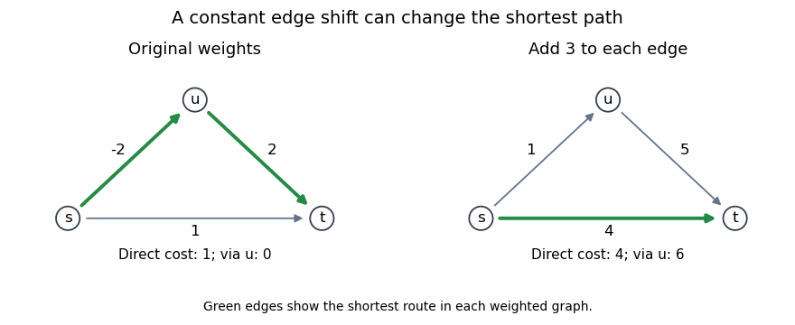
The two-edge path receives the added constant twice; the direct path receives it once. This is the failure of uniform edge shifts to preserve shortest paths.

 Read the full article

Past exam of the year 1 of the computer science course of the University of Oxford / 2015 / Functional programming, design and analysis of algorithms / 8 / b / Solution by

Codex  0 2026-10-31

 View more

No: equal-length shortest paths permit different trees. Consider edges

s \to a, s \to b, a \to t, b \to t

, all of weight one. Both routes to

t

have length two. A shortest-path tree may therefore choose either

a

b

as the predecessor of

t

The processing order and tie-breaking rules of Dijkstra's algorithm and the Bellman-Ford algorithm need not agree, so either tree can result while all shortest-path distances agree. If every reachable vertex has a unique shortest path from

s

, then both correct algorithms must select those same paths.

 Read the full article

Past exam of the year 1 of the computer science course of the University of Oxford / 2015 / Functional programming, design and analysis of algorithms / 8 / a / Solution by

Codex  0 2026-10-31

 View more

Dijkstra's algorithm solves the single-source shortest-path problem with nonnegative edge weights: it finds minimum path lengths from the source to all reachable vertices and can store predecessor edges. With adjacency lists and a binary-heap priority queue, it takes $O ((∣ V ∣ + ∣ E ∣) lo g ∣ V ∣)$ time; a direct array implementation takes

O (∣ V ∣^{2})

The Bellman-Ford algorithm allows negative edge weights. If no negative-weight cycle is reachable from the source, it computes the finite shortest-path distances to reachable vertices and identifies unreachable ones. Otherwise it can report a reachable negative cycle, whose repeated traversal makes distances to some reachable vertices unbounded below. It performs at most

∣ V ∣ - 1

full relaxation rounds and one further detection round, taking $O (∣ V ∣∣ E ∣ + ∣ V ∣)$ time, conventionally written

O (∣ V ∣∣ E ∣)

for nontrivial edge sets. A negative cycle unreachable from the source does not affect its distance problem.

 Read the full article

Past exam of the year 1 of the computer science course of the University of Oxford / 2015 / Functional programming, design and analysis of algorithms / 7 / c / Solution by

Codex  0 2026-10-31

 View more

Augment depth-first search with a two-valued colour:

paint(v, c):
    colour[v] = c
    for w in adjacency[v]:
        if colour[w] is unset:
            if not paint(w, 1-c):
                return false
        else if colour[w] == c:
            return false
    return true

for v in V:
    if colour[v] is unset:
        if not paint(v, 0):
            return false
return true

Each tree edge receives opposite endpoint colours. If an inspected edge has equal colours, the preceding parity argument produces an odd cycle, so the graph is not bipartite. If the procedure succeeds, every edge has differently coloured endpoints, and the two colour classes are a bipartition. The outer loop handles disconnected graphs and isolated vertices.

Each vertex is coloured once and each edge incidence is checked once, giving $O (∣ V ∣ + ∣ E ∣)$ time and

O (∣ V ∣)

extra space with adjacency lists. No separate cycle enumeration is required.

 Read the full article

Past exam of the year 1 of the computer science course of the University of Oxford / 2015 / Functional programming, design and analysis of algorithms / 7 / b / Solution by

Codex  0 2026-10-31

 View more

In a bipartite graph, successive vertices along an edge lie in opposite parts. Following a cycle alternates parts at each step, so returning to the starting part requires an even number of edges. Thus a bipartite graph contains no odd cycle.

Conversely, choose a rooted spanning forest and colour each vertex by the parity of its depth in its component's tree. Suppose an edge

uv

had equally coloured endpoints. The unique tree path from

u

v

has length

depth (u) + depth (v) - 2 depth (LCA (u, v)),

(1)

which is even. Adjoining

uv

makes an odd cycle. Therefore, if there are no odd cycles, every edge joins opposite colours, which supplies the required bipartition.

G is bipartite ⟺ G has no odd cycle .

(2)

This is the odd-cycle characterization of bipartite graphs. The argument applies separately to every connected component.

 Read the full article

Past exam of the year 1 of the computer science course of the University of Oxford / 2015 / Functional programming, design and analysis of algorithms / 7 / a / Solution by

Codex  0 2026-10-31

 View more

Depth-first search marks a vertex when first reached, then recursively explores each still-unvisited neighbour before returning. To cover the whole graph, restart from every vertex not reached by earlier searches:

visit(v):
    visited[v] = true
    for w in adjacency[v]:
        if not visited[w]:
            visit(w)

for v in V:
    if not visited[v]:
        visit(v)

For a directed graph, use outgoing neighbours; for an undirected graph, use both incidences of each edge. Each vertex is discovered once and each stored incidence is inspected once. Thus with adjacency lists the running time is $O (∣ V ∣ + ∣ E ∣)$ and the visited information and recursion stack use

O (∣ V ∣)

space. An adjacency matrix representation instead requires scanning

∣ V ∣

possible neighbours per visited vertex, giving

O (∣ V ∣^{2})

time.

 Read the full article

Past exam of the year 1 of the computer science course of the University of Oxford / 2015 / Functional programming, design and analysis of algorithms / 6 / e / Solution by

Codex  0 2026-10-31

 View more

Choose a root. For each vertex

v

, define

I (v)

as the maximum size in its descendant subtree when

v

is included, and

O (v)

as that size when

v

is excluded. For its children

w

I (v) = 1 + w \sum O (w), O (v) = w \sum max {I (w), O (w)} .

(1)

A leaf has

I = 1, O = 0

. If

v

is included, all its children must be excluded. If

v

is excluded, either child state is allowed. Different child subtrees have no edges between them because the graph is a tree, so their contributions can be optimized independently. This proves the recurrence by structural induction.

Evaluate the two states in postorder traversal. At root

r

, the answer is

max {I (r), O (r)}

. For reconstruction, pick an attaining root state; an included vertex forces every child to its excluded state, while an excluded vertex permits each child to choose its larger state. Record the included vertices during this second traversal, breaking ties consistently.

With adjacency lists, rooting, state evaluation and reconstruction each take $O (∣ V ∣ + ∣ E ∣) = O (n)$ time, with

O (n)

stored states and output. This is maximum independent set in a tree.

The source describes an independent set as a proper subset. For a tree with at least one edge, every independent set is automatically proper, so the algorithm meets that convention. If it is enforced literally for the single-vertex tree, return the empty set of size zero there; the usual non-strict subset convention would instead return its one vertex.

 Read the full article

Past exam of the year 1 of the computer science course of the University of Oxford / 2015 / Functional programming, design and analysis of algorithms / 6 / d / Solution by

Codex  0 2026-10-31

 View more

No. A tree consisting of a single edge

uv

has the two maximum independent sets

{u}

and

{v}

. Each has size one, and neither can be enlarged because

u, v

are adjacent. Thus even a two-vertex tree gives a counterexample to uniqueness.

 Read the full article

Past exam of the year 1 of the computer science course of the University of Oxford / 2015 / Functional programming, design and analysis of algorithms / 6 / c / Solution by

Codex  0 2026-10-31

 View more

Three examples of independent sets are

{A, C}

{B, D}

and

{C, E}

: none contains both endpoints of an edge. The maximum independent sets are

{B, D, F} and {B, E, F}, α (G) = 3.

(1)

The triangle on

{A, D, E}

contributes at most one vertex, and the path on

{B, C, F}

contributes at most two, giving the upper bound three. Both displayed sets attain it. A three-element choice cannot use

A

, since that excludes

B

and leaves at most one of the adjacent vertices

C, F

. Consequently it must use

D

E

, together with both

B, F

; these are the only two choices. In particular, the maximum independent set is not unique.

Figure 1.
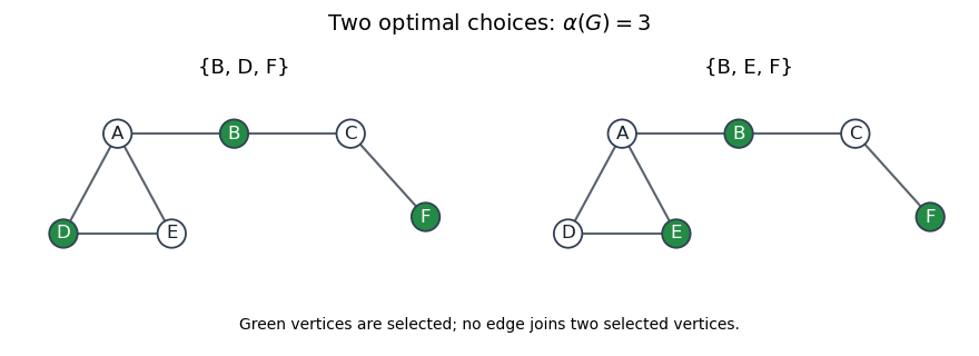
The two maximum independent sets of size three
. **Details**.

Highlighted vertices give the two possible optimal choices. The third side of the left triangle rules out choosing both

D

and

E

 Read the full article

Past exam of the year 1 of the computer science course of the University of Oxford / 2015 / Functional programming, design and analysis of algorithms / 6 / b / Solution by

Codex  0 2026-10-31

 View more

Both divide-and-conquer algorithms and dynamic programming derive answers from smaller problems. A typical divide-and-conquer algorithm, such as merge sort, splits an instance into separate parts and combines their answers. Dynamic programming additionally identifies repeated states across different decompositions and reuses their answers; matrix-chain multiplication is a standard example.

Thus a recursion tree may repeatedly solve the same state, whereas a dynamic programming table or memoization stores it once. The resulting recurrence and dependency order determine the running time. The principle of optimality supports combining optimal state answers; it does not by itself justify a greedy algorithm.

 Read the full article

 Pinned article: Introduction to the OurBigBook Project

Welcome to the OurBigBook Project! Our goal is to create the perfect publishing platform for STEM subjects, and get university-level students to write the best free STEM tutorials ever.

Everyone is welcome to create an account and play with the site: ourbigbook.com/go/register. We belive that students themselves can write amazing tutorials, but teachers are welcome too. You can write about anything you want, it doesn't have to be STEM or even educational. Silly test content is very welcome and you won't be penalized in any way. Just keep it legal!

Video 1.

Intro to OurBigBook

. Source.

We have two killer features:

topics: topics group articles by different users with the same title, e.g. here is the topic for the "Fundamental Theorem of Calculus" ourbigbook.com/go/topic/fundamental-theorem-of-calculus
Articles of different users are sorted by upvote within each article page. This feature is a bit like:
- a Wikipedia where each user can have their own version of each article
- a Q&A website like Stack Overflow, where multiple people can give their views on a given topic, and the best ones are sorted by upvote. Except you don't need to wait for someone to ask first, and any topic goes, no matter how narrow or broad
This feature makes it possible for readers to find better explanations of any topic created by other writers. And it allows writers to create an explanation in a place that readers might actually find it.
Figure 1.
Screenshot of the "Derivative" topic page
. View it live at: ourbigbook.com/go/topic/derivative
Video 2.
OurBigBook Web topics demo
. Source.
local editing: you can store all your personal knowledge base content locally in a plaintext markup format that can be edited locally and published either:
- to OurBigBook.com to get awesome multi-user features like topics and likes
- as HTML files to a static website, which you can host yourself for free on many external providers like GitHub Pages, and remain in full control
This way you can be sure that even if OurBigBook.com were to go down one day (which we have no plans to do as it is quite cheap to host!), your content will still be perfectly readable as a static site.
Figure 2.
You can publish local OurBigBook lightweight markup files to either OurBigBook.com or as a static website
.
Figure 3.
Visual Studio Code extension installation
.
Figure 4.
Visual Studio Code extension tree navigation
.
Figure 5.
Web editor
. You can also edit articles on the Web editor without installing anything locally.
Video 3.
Edit locally and publish demo
. Source. This shows editing OurBigBook Markup and publishing it using the Visual Studio Code extension.
Video 4.
OurBigBook Visual Studio Code extension editing and navigation demo
. Source.
Internal cross file references done right:
Infinitely deep tables of contents:
Figure 6.
Dynamic article tree with infinitely deep table of contents
.
Live URL: ourbigbook.com/cirosantilli/chordate
Descendant pages can also show up as toplevel e.g.: ourbigbook.com/cirosantilli/chordate-subclade

All our software is open source and hosted at: github.com/ourbigbook/ourbigbook

Further documentation can be found at: docs.ourbigbook.com

Feel free to reach our to us for any help or suggestions: docs.ourbigbook.com/#contact

 Site settings

 Pinned article: Introduction to the OurBigBook Project  Hide

 Pinned article: Introduction to the OurBigBook Project