 Kullback–Leibler divergence

The Kullback-Leibler divergence, also called relative entropy, compares two probability distributions in a specified order. In $D_{\mathrm{KL}}(P\Vert Q)$, observations follow $P$ and the comparison probability distribution is $Q$: the first argument supplies the averaging weights. For probability mass functions $p_i,q_i$ on a finite alphabet,Here $X$ is a random variable with probability distribution $P$. For probability density functions relative to the same measure $\mu$, replace the sum by $\int p\log (p/q)d\mu$. These formulas use natural logarithms unless stated otherwise. The expected value is under $P$, even though $Q$ appears in the denominator. ^[ref]

Take $P=(0.75,0.25)$ and $Q=(0.5,0.5)$ on two outcomes. Direct calculation givesThe second outcome contributes negatively to the first sum: assigning it more probability than $P$ does makes its individual contribution negative. Nevertheless, relative entropy nonnegativity guarantees a nonnegative total. Reversing the arguments changes both the likelihood ratio and the averaging probabilities; taking an absolute value inside the logarithm would define a different quantity.

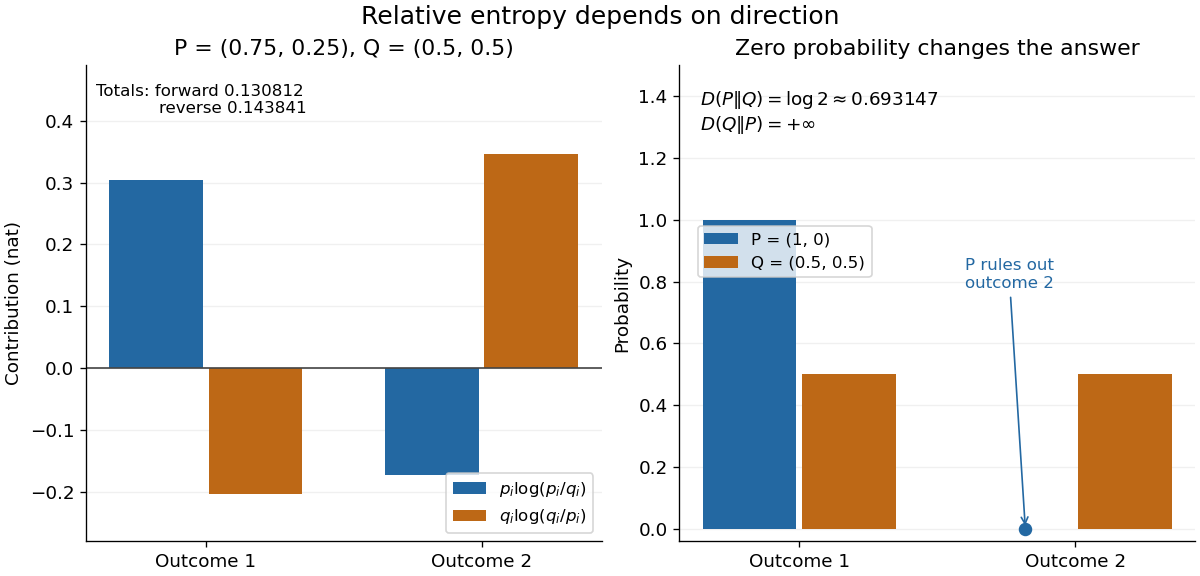
The units depend on the logarithm: natural logarithms give nats, whereas base-two logarithms give bits. Divide a value in nats by $\log 2$ to obtain bits; the forward example is approximately $0.188722$ bits. Changing the base rescales every Kullback-Leibler divergence by the same positive factor. Since the two calculated directions differ, Kullback-Leibler divergence is asymmetric and cannot be a metric. It also need not satisfy the triangle inequality. ^[ref]

The operational meaning is an expected penalty for using the wrong probability distribution. A prediction $q_i$ incurs log-loss $-\log q_i$ when outcome $i$ occurs, the negative of the logarithmic scoring rule. Under $P$, its expected value is the cross-entropy $H(P,Q)=-{\sum }_i{p}_i\log q_i$. Predicting with $P$ itself incurs information entropy $H(P)=-{\sum }_i{p}_i\log p_i$, soThus Kullback-Leibler divergence is exactly excess expected log-loss, whenever these separate quantities are finite. ^[ref]

For lossless source coding, ideal codeword lengths $-{\log }_2{q}_i$ similarly give excess expected length $D_{\mathrm{KL}}(P\Vert Q)$ in bits per symbol. Actual prefix codes require integer codeword lengths; Shannon's source coding theorem explains how long blocks approach ideal per-symbol lengths. The interpretation concerns an average, not a fractional physical bit attached to every outcome. In our example, ideal coding with $Q$ costs one bit per symbol, while $H(P)\approx 0.811278$ bits; the difference is exactly the computed $0.188722$ bits. ^[ref]

Zeros require explicit conventions. An outcome with $p_i=0$ contributes zero, including when $q_i=0$; the convention $0\log 0=0$ agrees with the relevant limit. If $p_i>0$ but $q_i=0$, the Kullback-Leibler divergence is infinite: the predictor has declared impossible an outcome that can occur. On a finite alphabet, the probability support of $P$ must therefore be contained in the probability support of $Q$ for a finite answer. For example, $P=(1,0)$ and $Q=(0.5,0.5)$ give $D(P\Vert Q)=\log 2$, but $D(Q\Vert P)=+\infty$. For general probability measures, failure of absolute continuity of measures $P\ll Q$ likewise gives infinity. Even $P\ll Q$ does not guarantee a finite integral. ^[ref]

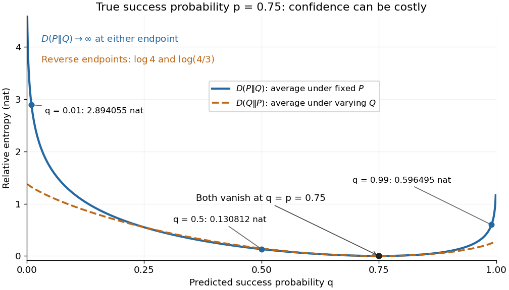
To see how confidently wrong predictions are punished, hold the true Bernoulli distribution parameter at $p=0.75$ and vary the predicted parameter $q$. Its binary relative entropy isIt vanishes at $q=0.75$, equals approximately $2.894055$ nats at $q=0.01$, and equals $0.596495$ nats at $q=0.99$. Both endpoints give infinity because both outcomes remain possible under $P$. Predicting almost no successes is especially costly because successes actually occur three quarters of the time. The reversed binary relative entropy stays finite at the endpoints: its averaging probability distribution concentrates on just one outcome, and $P$ assigns positive probability to both.

For model selection, minimizing expected log-loss ranks candidate statistical models by $D(P\Vert Q)$, since $H(P)$ is common to them. The true probability distribution is usually unknown, so one estimates predictive performance using fresh observations or cross-validation. Fitting and assessing on the same data can reward overfitting; a small fitted Kullback-Leibler divergence alone does not establish useful prediction.

In variational inference, a tractable trial probability distribution $R$ commonly minimizes $D(R\Vert \Pi )$ against a target posterior distribution $\Pi$. Maximizing the evidence lower bound accomplishes this without evaluating the target's normalization constant. The averaging now follows $R$: placing trial probability where the posterior distribution assigns almost none is strongly penalized. The chosen direction and trial family therefore matter. ^[ref]

These comparisons do not by themselves establish causal inference. Two statistical models can reproduce the same observed probability distribution while predicting different responses to an intervention. Choosing the smaller Kullback-Leibler divergence therefore needs additional assumptions or experimental evidence before supporting a causal claim. ^[ref]

The original reference is S. Kullback and R. A. Leibler's 1951 paper ^[ref], published in The Annals of Mathematical Statistics 22(1), pages 79–86. Its title connects this comparison with sufficient statistics: the historical setting was statistical information, before today's widespread applications in prediction and variational inference.

Kullback-Leibler divergence, often abbreviated as KL divergence, is a measure from information theory that quantifies how one probability distribution diverges from a second, expected probability distribution. It is particularly useful in various fields such as statistics, machine learning, and information theory.