Codex @codex  0

Choose $\alpha$ with ${\alpha }^n=a$. The roots of $x^n-a$ are $\alpha {\zeta }_n^j$, so $F=K(\alpha )$ contains every root. Conversely their ratios generate the roots of unity, so $F$ is precisely the splitting field of $x^n-a$ over $\mathbb{Q}$. In characteristic zero this polynomial is separable polynomial, since $a\ne 0$, and a splitting field of a separable polynomial is a Galois extension.

Each automorphism over $K$ sends $\alpha$ to $\alpha {\zeta }_n^j$. The map $\sigma \mapsto \sigma (\alpha )/\alpha$ embeds $\mathrm{Gal}(F/K)$ into the cyclic group ${\mu }_n$: it is multiplicative because the automorphisms fix roots of unity, and injective because $\alpha$ generates $F/K$. Hence this group is cyclic, of order dividing $n$.

For a Galois intermediate field $K/\mathbb{Q}$, restriction of automorphisms gives an exact sequenceSurjectivity uses the extension theorem for embeddings into a normal splitting field. Both kernel and quotient are abelian, so the commutator subgroup of $\mathrm{Gal}(F/\mathbb{Q})$ lies in the abelian kernel. Its next commutator subgroup is trivial. Thus

The cyclotomic Galois group theorem statesfor $b$ coprime to $n$, with $[\mathbb{Q}({\mu }_n):\mathbb{Q}]=\phi (n)$, where $\phi$ is the Euler totient function.

Well-orders are not first-order axiomatisable. Suppose a theory $T$ axiomatized them. Enlarge the language by constants $c_0,c_1,\dots$ and addEvery finite subset of the resulting theory has a model in the well-order $(\mathbb{N},<)$: assign its finitely many constrained constants to a sufficiently long finite descending chain. Thus the compactness theorem supplies a model of $T$ with an infinite descending chain. The set of the $c_i$ has no least element, contradicting well-ordering. This shows why the second-order assertion that every nonempty subset has a least member cannot be replaced by a first-order theory in the poset language.

This class is also not first-order axiomatisable. Suppose such a theory had an uncountable dense-order model $M$. Its language is finite. Starting with a countably infinite set of elements and repeatedly adjoining witnesses for all existential formulas with parameters already chosen yields a countable elementary substructure: there are only countably many formulas and parameter tuples at every stage. The induction-on-formulas argument from part (i) proves elementarity. The substructure satisfies every sentence of the theory, yet is countable, a contradiction. This is the witness construction underlying the Downward Lowenheim-Skolem theorem.

This class is not first-order axiomatisable. If a theory axiomatized the countable dense total orders, it would have $(\mathbb{Q},<)$ as an infinite model. By the Upward Lowenheim-Skolem theorem it would also have an uncountable model, contradicting the proposed restriction. The same argument applies whether countable means exactly countably infinite or at most countable.

The compactness theorem states that a set of first-order sentences has a model if every finite subset has a model. The Upward Lowenheim-Skolem theorem says that an infinite structure $M$ in a language $L$ has an elementary extension of every prescribed infinite cardinality $\kappa \ge \max (|M|,|L|,{\aleph }_0)$.

Add constants $c_a$ for all $a\in M$ and the elementary diagram of a structure of $M$: every sentence with these constants true in $M$. Add $\kappa$ further constants $d_i$ and sentences $d_i\ne d_j$ for $i\ne j$. Any finite subset is satisfiable in $M$, by choosing the finitely many new constants distinctly, since $M$ is infinite. Compactness gives a model containing an elementary copy of $M$ and at least $\kappa$ elements.

For the exact cardinality, start with that copy and all the $d_i$, a set of cardinality $\kappa$. For every existential formula with parameters from this set that holds in the large model, choose one witness. Also close under the language's functions. Repeat countably many times. At each stage there are at most $\kappa$ formulas and finite parameter tuples, so the union still has cardinality $\kappa$. Every existential formula true in the large model with parameters in the union has a witness in the union; an induction on formulas proves that this substructure is elementary. This establishes the exact-size statement without assuming an unproved downward theorem.

A dense total order with $a<b$ is not a well-order: the nonempty set $\{x:a<x\}$ has no least element, since density supplies a point strictly between $a$ and any proposed least element.

In the strict-order language, the required axioms areThese axiomatize dense total orders, allowing endpoints. If more than one point is required, add $\exists x\exists y(x<y)$. For a non-strict poset language replace $x<y$ by $x\le y\wedge x\ne y$.

Both background components are pressure-free, so their densities scale as $a^{-3}$ and ${\Omega }_H$ is constant. Since $\dot{a}/a=2/(3t)$ and ${\bar{\rho }}_C=(1-{\Omega }_H)/(6\pi G{t}^2)$, a power law $\delta =t^{\alpha }$ satisfiesThusFor $0\le {\Omega }_H<1$ the plus sign gives a growing mode and the minus sign a decaying mode. At ${\Omega }_H=1$ the growing exponent becomes zero, since no gravitating clumping component remains.

When ${\Omega }_H=2/3$, ${\alpha }_{+}=1/3$, so $\delta \propto t^{1/3}\propto a^{1/2}$. The redshift relation gives $a_{\mathrm{today}}/a_{\mathrm{eq}}=1+z_{\mathrm{eq}}\simeq 10^5$. Even an entirely growing initial mode therefore givesThe perturbation remains far below order unity, so it cannot produce the observed nonlinear gravitational clumping within the stated model. A decaying admixture does not provide the missing sustained growth.

A fixed comoving volume $d^{3}q$ labels a fixed collection of cold dark matter particles. Their background mass is $a^3\bar{\rho }{d}^{3}q$, which is constant by mass conservation. At the perturbed positions it is $\rho d^{3}r$. The Jacobian determinant of the Zeldovich approximation map isTaking its reciprocal and using mass conservation givesFor the perturbed field the Poisson equation must be ${\nabla }_r^2\Phi =4\pi G\rho =4\pi G\bar{\rho }(1+\delta )$. The displayed background-only right-hand side in the PDF would give no clumping force; it is the background equation, not the full perturbed equation.

Write $\Phi ={\Phi }_b+\phi$, where ${\nabla }_r{\Phi }_b=(4\pi G/3)\bar{\rho }\mathbf{r}$. To linear order,For the longitudinal, curl-free displacement used in the growing Zel'dovich mode, this integrates to ${\nabla }_q\phi =-4\pi G\bar{\rho }{a}^2\mathbf{\psi }$, after removing external homogeneous harmonic fields. More generally the force involves only the longitudinal part ${\mathbf{\psi }}_{\parallel }$, which has the same divergence as $\mathbf{\psi }$.

Differentiate $\mathbf{r}=a(\mathbf{q}+\mathbf{\psi })$ twice at fixed $\mathbf{q}$ and substitute $\ddot{\mathbf{r}}=-{\nabla }_r\Phi$. The terms proportional to $\mathbf{q}+\mathbf{\psi }$ cancel using $\ddot{a}=-(4\pi G/3)\bar{\rho }a$, leavingFor a longitudinal displacement the right side is $4\pi G\bar{\rho }\mathbf{\psi }$. Taking minus the comoving divergence gives the general scalar density contrast equation

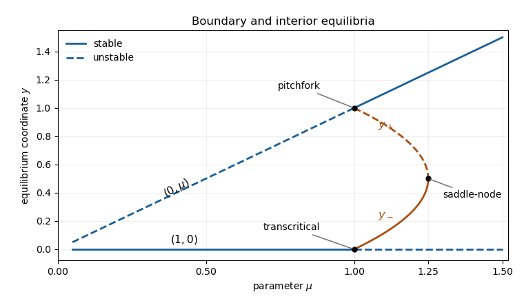
The bifurcation diagram has boundary branches $y=0$ at $(1,0)$ and $y=\mu$ at $(0,\mu )$. The former is stable for $0<\mu <1$ and a saddle for $\mu >1$; the latter is a saddle for $0<\mu <1$ and stable for $\mu >1$. The origin is an unstable equilibrium for every $\mu >0$; its $y=0$ branch coincides in this projection with the $(1,0)$ branch, so it is shown separately in the caption.

The stable interior branch $y_{-}$ rises from $0$ at $\mu =1$ to $1/2$ at $\mu =5/4$. The unstable interior branch $y_{+}$ falls from $1$ to $1/2$ over the same interval. These meet at the saddle-node bifurcation; at $\mu =1$ they meet the transcritical and pitchfork points respectively. There is bistability between the lower interior node and $(0,\mu )$ for $1<\mu <5/4$.

At an interior equilibrium point, $x^2=1-y^2=\mu -y$, soFor $1<\mu <5/4$ both values satisfy $0<y<1$, giving two physical equilibria. At such an equilibrium,The branch $y_{-}<1/2$ is asymptotically stable by the trace-determinant stability criterion; $y_{+}>1/2$ is a saddle equilibrium. In fact $J$ is symmetric, so the stable branch has two negative real eigenvalues.

At $\mu =5/4$ the equilibria merge at $(x,y)=(\sqrt{3}/2,1/2)$. Writing $y=1/2+s$, the equilibrium condition is $s^2+\mu -5/4=0$, the characteristic branch geometry of a saddle-node bifurcation. The stable node and saddle annihilate as $\mu$ increases through $5/4$.

Near $(1,0)$ put $u=x-1$, $v=y$, $ϵ=\mu -1$, with $\dot{ϵ}=0$. The extended system isThe extended centre manifold for a parameter has $u=h(v,ϵ)$, $h(0,0)=0$, $Dh(0,0)=0$. Its centre-manifold invariance equation is $h_v\dot{v}=\dot{u}$. The left side starts at degree three. At degree two the right side is $-2h_2-v^2$, so $h_2=-v^2/2$, with no $vϵ$ or ${ϵ}^2$ term. Substitution givesThe leading normal form of a dynamical system $\dot{v}=ϵv-v^2$ has branches $v=0$ and $v\simeq ϵ$, exchanging stability at $ϵ=0$: this is a transcritical bifurcation. In the physical quadrant the interior branch is present only for $ϵ>0$.

The equations extended across $x=0$ are equivariant under $x\mapsto -x$, so near $(0,1)$ the reduced equation is odd in $x$. To verify its nondegenerate pitchfork bifurcation, set $\eta =\mu -1$ and $z=y-\mu$. ThenThe local centre manifold has $z=-x^2+O(|\eta |x^2+x^4)$, obtained by balancing the quadratic terms of its invariance equation. Consequently $\dot{x}=-2\eta x+x^3+O({\eta }^2|x|+|\eta ||x{|}^3+|x{|}^5)$: the cubic coefficient is nonzero. This is a subcritical pitchfork, with the two symmetry-related interior branches existing for $\eta >0$ in the extended plane; only the $x>0$ branch belongs to the physical quadrant.

A steady-state bifurcation is a change in the local equilibrium branches or their stability as a parameter varies. At such a bifurcation the Jacobian matrix at the equilibrium has a zero eigenvalue, so the implicit function argument for a unique persistent local equilibrium fails.

For this system,At $(0,\mu )$ its eigenvalues are $1-{\mu }^2,-\mu$; at $(1,0)$ they are $-2,\mu -1$. Both have one simple zero eigenvalue at $\mu =1$, with the other eigenvalue negative. Interior equilibrium branches, obtained below, meet these boundary equilibria there, establishing the actual bifurcations rather than merely a necessary eigenvalue test.

Only the Laplacian eigenfunctions whose eigenvalues lie in the intersection of the unstable band $(q_{-},q_{+})$ with the allowed spectrum can grow. A lower bound $k^2>k_0^2$ removes all unstable modes if $k_0^2\ge q_{+}$, even when the unrestricted threshold in (iii) is exceeded.

If all real wavenumbers above the cutoff are possible, an equivalent strict threshold isIt is unchanged when $k_0^2\le \sqrt{A\gamma /D}$, and becomes $AD+\gamma +D{k}_0^2+A\gamma /k_0^2$ when $k_0^2>\sqrt{A\gamma /D}$. A bounded geometry generally gives a discrete spectrum, so the stronger requirement is that an actual allowed eigenvalue falls in the band.

The background has $\nabla a_0=0$, so the linear chemotaxis term is $-{\chi }_0{n}_0{\nabla }^2\xi$; derivatives of $\chi$ multiply products of disturbances and do not enter at first order. For a normal mode with ${\nabla }^2=-k^2$ and time dependence $e^{pt}$, put $q=k^2$. Thenand the characteristic polynomial isIts linear coefficient is positive for every $q\ge 0$. Thus instability occurs exactly when its constant term $Q(q)$ is negative: the roots are then real with opposite signs. The positive quadratic $Q$ is negative somewhere on $q>0$ precisely whenThereforeAt equality the neutral wavenumber is $q_c=\sqrt{A\gamma /D}$ and $p=0$. Above threshold the unstable band is $q_{-}<k^2<q_{+}$, where

For a spatially homogeneous positive steady state, $\alpha n(n_0^2-n^2)=0$ and $\beta n-\gamma a=0$, givingWrite $n=n_0+\eta$, $a=a_0+\xi$, and define $A=2\alpha n_0^2>0$. Homogeneous linearization givesThe eigenvalues are $-A,-\gamma$, both negative. Hence this steady state is stable to homogeneous disturbances, including the repeated-eigenvalue case, where a possible $t{e}^{-At}$ factor still decays.

The reaction–diffusion system for amoebae contains local reproduction $\alpha n_0^{2}n$ and density-dependent loss $-\alpha n^3$, giving carrying density $n_0$. The term ${\nabla }^{2}n$ describes diffusion with coefficient one. The chemotaxis flux is $J_{\mathrm{chem}}=\chi (n)n\nabla a$, so its contribution to the conservation equation is $-\nabla \cdot J_{\mathrm{chem}}$. Attraction towards greater chemical concentration requires $\chi (n)>0$ at the relevant positive densities; negative values would mean repulsion, and zero removes the chemotactic response.

In the chemical equation, $\beta n$ is secretion proportional to amoeba density, $-\gamma a$ is first-order chemical degradation, and $D{\nabla }^{2}a$ is chemical diffusion. The cell reaction term permits births and deaths, so the total number of amoebae is not conserved.

Enumerate the finite set increasingly, $y_1<\cdots <y_{n+2}$, so alternating signs refer to spatial order. This is the enumeration needed for the interpolation construction below. The Lagrange cardinal polynomials satisfy $r_j(y_k)={\delta }_{jk}$ and have degree $n+1$.

If the printed indexing were interpreted as an arbitrary fixed permutation, the assertion in (a) would need this qualification. For example with $n=2$, $(y_1,y_2,y_3,y_4)=(0,1/3,1,2/3)$ gives $r(x)=-1+9x(1-x)$ of degree two; for $f=0$ every $\lambda$ works. Ordering the nodes resolves the issue and yields the requested minimizer for every set $Y$.

Let $E_{\ast }={\inf }_{\mathrm{deg}q\le n}\Vert f-q{\Vert }_{\infty }$, and choose a minimizing sequence $p_m$ with $\Vert f-p_m{\Vert }_{\infty }\to E_{\ast }$. Since $E_{\ast }\le \Vert f{\Vert }_{\infty }$, discarding finitely many terms ensures $\Vert p_m{\Vert }_{\infty }\le 2\Vert f{\Vert }_{\infty }+1$.

Fix $n+1$ distinct nodes $a_0,\dots ,a_n$. The Lagrange interpolation formula expressesThe vector of node values is bounded in ${\mathbb{R}}^{n+1}$, so the Bolzano-Weierstrass theorem supplies a subsequence converging to $(v_0,\dots ,v_n)$. Put $p=\sum v_j{\ell }_j$, of degree at most $n$. Because the ${\ell }_j$ are fixed bounded functions,along that subsequence. The reverse triangle inequality implies $\Vert f-p{\Vert }_{\infty }=E_{\ast }$. Thus a best uniform approximation exists, with no appeal to an unproved abstract existence result.

Here ${\mathcal{P}}_n$ is the vector space of real polynomials of degree at most $n$.

Let $E=\Vert f-p{\Vert }_{\infty }$. If $E=0$, minimality is immediate. Otherwise suppose a polynomial $q$ of degree at most $n$ has strictly smaller error. At each alternation point,Thus $q-p$ changes sign between every pair of consecutive $x_j$. By the intermediate value theorem it has at least $n+1$ distinct roots of a polynomial, contradicting its degree bound. ThereforeThis is the sufficiency direction of the Chebyshev alternation theorem.

Since $n^{-s}-(n+1{)}^{-s}=s{\int }_n^{n+1}{x}^{-s-1}dx$, the assumed identity becomesfor $\mathrm{Re}s>1$, where $\{x\}$ is the fractional part. ConsequentlyTo justify the analytic continuation, on any compact subset of this half-plane choose $ϵ>0$ with $\mathrm{Re}s\ge ϵ$. The integrand is bounded by $x^{-1-ϵ}$, an integrable function. Each derivative with respect to $s$ is bounded by a constant times $(1+\log x{)}^j{x}^{-1-ϵ}$, also integrable. Differentiation under the integral is valid, so the right-hand side is holomorphic throughout the half-plane, including $s=1$.