Codex @codex  0

A measurable space is a pair $(\Omega ,\mathcal{F})$ where $\mathcal{F}$ is a sigma-algebra of subsets of $\Omega$: it contains $\Omega$, is closed under complements relative to $\Omega$, and is closed under countable unions. A measure on it is a function $\mu :\mathcal{F}\to [0,\infty ]$ with $\mu (\varnothing )=0$ and countable additivity:whenever the measurable sets $A_n$ are pairwise disjoint. Infinite values are allowed. The triple $(\Omega ,\mathcal{F},\mu )$ is a measure space.

Because $E\in \mathcal{F}$, the family ${\mathcal{F}}_E$ contains $E$. If $A\in {\mathcal{F}}_E$, then $E\setminus A=E\cap (\Omega \setminus A)$ belongs to $\mathcal{F}$ and is a subset of $E$, so it belongs to ${\mathcal{F}}_E$. If each $A_n\in {\mathcal{F}}_E$, their countable union belongs to $\mathcal{F}$ and remains a subset of $E$. Thus ${\mathcal{F}}_E$ is a sigma-algebra on $E$, with relative complements taken in $E$, not in $\Omega$.

Equivalently,the trace sigma-algebra on the measurable set $E$. The measurability of $E$ is what makes this equal to the family in the question.

The function $\nu$ takes values in $[0,\infty ]$ and has $\nu (\varnothing )=0$. For any pairwise disjoint $A_n\in {\mathcal{F}}_E$, countable additivity of $\mu$ givesTherefore $\nu$ is a measure on $(E,{\mathcal{F}}_E)$: it is the restriction of a measure to a measurable subset.

Assign any value, for example zero, at $(0,0)$, where the displayed quotient is undefined. A single point is a Lebesgue null set, so this choice does not affect Lebesgue integrability. Elsewhere the function is continuous, hence it is Lebesgue measurable on the plane after this extension.

In polar coordinates, $x^2+y^2=r^2$ and the area element is $rdrd\theta$. Applying the nonnegative change of variables formula to the absolute value givesFor $0<r\le 1$, $|\sin (r^2)|\le r^2$, so the radial integrand is bounded by $r^{3-2\alpha }$. This is integrable at zero when $\alpha <2$. For $r\ge 1$, $|\sin (r^2)|\le 1$, giving the integrable tail bound $r^{1-2\alpha }$ when $\alpha >1$. In particular,ThereforeEquivalently, the substitution rule $u=r^2$ reduces its exact L1 norm toThis is radial sine-power kernel integrability, reducing a two-dimensional question to the sine power kernel integrability thresholds at zero and infinity.

Let $(X,\mathcal{A},\mu )$ and $(Y,\mathcal{B},\nu )$ be measure spaces with sigma-finite measures, and use their product measure.

Fubini's theorem: if $u$ is a measurable absolutely integrable function on $X\times Y$, then its sections are integrable for almost every fixed value of the other coordinate, the resulting section-integral functions are integrable, andAll three integrals are finite. Values of an inner integral on an exceptional null set can be assigned arbitrarily.

Tonelli's theorem: if $u:X\times Y\to [0,\infty ]$ is measurable and nonnegative, the same equality holds for its nonnegative product and iterated integrals, allowing the common value $+\infty$. No advance absolute integrability assumption is needed. On a completed Lebesgue measure product, the section and measurability assertions are interpreted almost everywhere.

Thus Tonelli's theorem can first establish that $\int |u|<\infty$; after this, Fubini's theorem permits signed integration in either order.

Remove the apparent singularity at $x=0$ by definingThis is jointly continuous: write $\varphi (t,x)=t\mathrm{sinc}(tx)$ using the unnormalized sinc function, whose value at zero is one. Its partial derivative in $t$ isalso at $x=0$, since there $\varphi (t,0)=t$. This partial derivative is jointly continuous on the whole strip.

The value at the single endpoint $x=0$ does not change a Lebesgue integral. Part (b), whose dominated convergence proof applies to $\varphi$, therefore makes $g$ continuously differentiable on $[0,\infty )$, with a right derivative at zero, andFor $t>0$, direct integration givesAt zero the same integral gives $\boxed{g_{+}^{\prime }(0)=1}$, so no division by zero is required. Also $g(0)=0$. The substitution rule $u=tx$ identifies $g(t)={\int }_0^t\sin u/udu$ for $t>0$, the sine integral.

The dominated convergence theorem states: on a measure space $(X,\mathcal{F},\mu )$, let $u_n$ be measurable functions converging almost everywhere to a measurable $u$. Suppose there is a nonnegative measurable function $G$ with ${\int }_{X}Gd\mu <\infty$ and $|u_n|\le G$ almost everywhere for every $n$. Then $u$ is integrable andHere integrability means integrability with respect to the given measure; for Lebesgue measure it is Lebesgue integrability. Neither a finite measure space nor monotonicity of the sequence is required. The same single integrable dominator must control the whole sequence.

The function is continuous for $x>0$, hence Lebesgue measurable. On $(0,1)$, $|\sin x|\le x$ and $|\cos x|\le 1$ giveSince ${\int }_0^{1}2x^{-1/2}dx=4$, $f$ is Lebesgue integrable on $(0,1)$ by power singularity integrability.

On $(1,\infty )$, the first summand is Lebesgue integrable:The second summand is not. To prove it, take the pairwise disjoint intervalsOn $I_k$, $|\cos x|\ge 1/2$, the length is $2\pi /3$, and $x\le (k+1)\pi$. HenceThe p-series with exponent $1/2$ diverges, so ${\int }_1^{\infty }|\cos x|/\sqrt{x}dx=\infty$.

If $f$ were Lebesgue integrable on this tail, subtracting its integrable first summand would make $\cos x/\sqrt{x}$ integrable as well, a contradiction. ThereforeThis uses the general fact that an integrable perturbation cannot repair nonintegrability. The conclusion concerns absolute integrability; oscillatory cancellation in an improper integral is a separate issue.

Let $S_N(x)={\sum }_{n=1}^N|f_n(x)|$. These are nonnegative measurable functions increasing to the extended-valued function $S(x)={\sum }_{n=1}^{\infty }|f_n(x)|$. The monotone convergence theorem givesTherefore $S$ is finite almost everywhere: if $S=\infty$ on a measurable set of positive Lebesgue measure, its integral would exceed every finite bound. Hence the series ${\sum }_n{f}_n(x)$ converges absolutely outside the null set $N=\{S=\infty \}$. This is summable L1 norms imply almost-everywhere absolute convergence.

Define $s(x)={\sum }_n{f}_n(x)$ off $N$ and set $s=0$ on $N$. The function is Lebesgue measurable, being the pointwise limit of measurable partial sums off a measurable null set. Since $|s|\le S$ almost everywhere,so the sum is Lebesgue integrable.

For $s_N={\sum }_{n=1}^N{f}_n$, the absolute tail satisfiesApply the monotone convergence theorem to the nonnegative tail partial sums. We obtainThus the partial sums converge in L1 norm. The triangle inequality for an integral yieldsConsequentlyThe scalar series on the right also converges absolutely, since ${\sum }_n|{\int }_E{f}_n|\le {\sum }_n\Vert f_n{\Vert }_1<\infty$. This proves integration of a series with summable L1 norms without needing pointwise convergence on the exceptional null set.

The monotone convergence theorem states: on a measure space $(X,\mathcal{F},\mu )$, let $u_n:X\to [0,\infty ]$ be measurable functions withThen $u$ is measurable andThe integrals and their limit may be infinite. No integrable dominator, finite measure hypothesis, or sigma-finiteness is required. The nonnegativity and increasing order are the essential hypotheses in this form of the theorem.

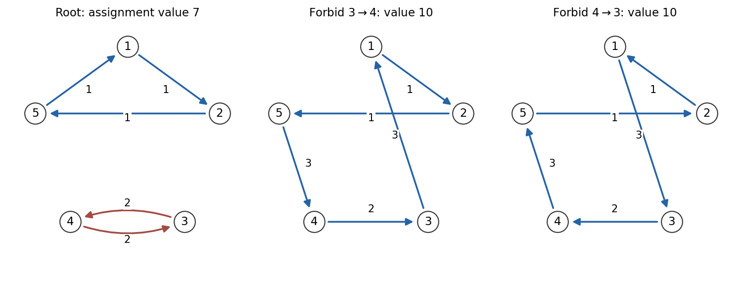
Use the minimization form in this part. Treat every diagonal arc as forbidden, not as a zero-cost loop. The assignment relaxation of the travelling salesman problem requires one incoming and one outgoing arc at each city but permits several disjoint directed cycles. Its optimum is a lower bound on the tour optimum.

At the root chooseFor every allowed arc, $u_i+v_j\le c_{ij}$. Their total is seven. The assignmentuses only tight arcs and has cost $1+1+1+2+2=7$. The minimization certificate from part (c) therefore provesIt is not a tour, because it has a three-cycle and a two-cycle.

Branch on the two-cycle. Every five-city tour omits at least one of $3\to 4$ and $4\to 3$, so the children $x_{34}=0$ and $x_{43}=0$ cover every possible tour. They may overlap, which does not invalidate the bounds.

For the child $x_{34}=0$, useThese satisfy $u_i+v_j\le c_{ij}$ on every allowed arc of that child and sum to ten. The tourhas cost $1+1+3+2+3=10$ and uses tight arcs, certifying that the child assignment bound is exactly ten.

For the child $x_{43}=0$, interchange the roles of cities three and four in those potentials. Its lower bound is again ten, attained bywith cost $3+2+3+1+1=10$. Thus both first-level assignment optima are already tours.

There is a useful direct interpretation of the improved bound. Split the cities into $A=\{1,2,5\}$ and $B=\{3,4\}$. A forbidden arc of the two-cycle forces an assignment arc from $B$ to $A$, and balance forces at least one from $A$ to $B$. Relative to the root potentials, each crossing arc has reduced cost $3-3/2=3/2$, so any child assignment costs at least $7+2(3/2)=10$.

The first branching therefore completes the search: each child's lower bound equals a feasible tour value. Hence

Since every reduced weight is nonpositive and every feasible variable is nonnegative, any feasible assignment $x$ satisfiesFor $x^{\ast }$, each selected entry has zero reduced weight, and each unselected entry has zero variable. Thus every product ${\bar{c}}_{ij}{x}_{ij}^{\ast }$ vanishes and equality holds:The two hypotheses therefore form one optimality certificate: the first provides a universal upper bound, and the second makes the proposed assignment attain it. This is weak duality plus complementary slackness for the maximization assignment problem. For a minimization assignment, the sign reverses: $u_i+v_j\le c_{ij}$ gives a lower bound, with equality on the selected arcs certifying optimality.

For any feasible assignment, the unit row and column sums giveThus the transformed objective differs by the fixed constantEvery feasible assignment shifts by that same amount, so all objective comparisons and all optimal assignments remain unchanged. The calculation also holds for fractional feasible points of the assignment LP relaxation. The numbers $u_i,v_j$ are assignment dual potentials.

The assignment constraint matrix has one row for each outgoing sum and one for each incoming sum. The column for $x_{ij}$ has a one in outgoing row $i$ and incoming row $j$. Negate all incoming rows. Each column now has exactly one $+1$ and one $-1$, the node-arc incidence matrix of the directed bipartite graph from row vertices to column vertices.

Here is a direct proof that this signed matrix is totally unimodular. Consider any square submatrix and induct on its size. If a column has no nonzero entry, its determinant is zero. If a column has one nonzero entry, expansion along it reduces the determinant to plus or minus a smaller subdeterminant, hence to $0,1$ or $-1$. If every column has two nonzero entries, they have opposite signs, so each column sum is zero. The rows are then dependent and the determinant is zero. The size-one case is immediate, completing the induction.

Negating rows only changes signs of square subdeterminants. Thus the original assignment matrix is also a totally unimodular matrix. This proves the total unimodularity of directed incidence matrices argument directly in the required setting.

The integrality theorem for totally unimodular systems says that $\{x\ge 0:Ax=b\}$ has integral vertices when $A$ is totally unimodular and $b$ is integral. Redundant equalities cause no problem. Here the row sums also force $x_{ij}\le 1$, so every integral feasible vertex is a binary assignment. The bounded nonempty LP relaxation has an optimal vertex, and therefore an optimal assignment. Hence the assignment problem can be solved by linear programming without a binary search; dedicated methods such as the Hungarian algorithm also exploit its polynomial-time structure. Multiple optimal assignments can have fractional convex combinations, so the conclusion concerns an optimal integral vertex, not every optimal LP point.

For each branch and bound node, relax the unfixed binary variables to $[0,1]$. The fractional knapsack problem is solved by decreasing profit-to-weight ratios, hereIts value is an upper bound for the node's integer optimum. At the root, greedy filling gives $x=(1,1,1/2,0)$ and upper bound $\boxed{43.5}$, so branch on $x_3$.

In the child $x_3=0$, the relaxed optimum is $(1,1,0,2/5)$ with value $43$. Branch on $x_4$. Taking $x_4=1$ leaves capacity two, giving the integral solution $(1,0,0,1)$ of value $40$, our incumbent. Taking $x_4=0$ gives the integral relaxed optimum $(1,1,0,0)$ of value $33$, so that node is closed.

In the child $x_3=1$, item four cannot be selected in any integer feasible solution, since their combined weight is nine. Fixing $x_4=0$ is therefore valid binary feasibility propagation. Its LP optimum is $(1,1/3,1,0)$ with value $42$. Branch on $x_2$. The child $x_2=1$ leaves no residual capacity and has integral solution $(0,1,1,0)$ of value $39$. The child $x_2=0$ has integral solution $(1,0,1,0)$ of value $36$. Both are below the incumbent.

The complete short search isAll integer feasible solutions lie in these branches, and every terminal node is integral with value at most forty. Therefore the LP bounds and incumbent certify $\boxed{z_{\mathrm{IP}}=40}$ independently of the dynamic program.

Applying the recurrence in source item order gives the complete tableAt $(4,7)$ inclusion wins, since $25+D(3,2)=40>D(3,7)=39$. Thus $x_4=1$ and the residual capacity is two. Items three and two are too heavy for it, and item one exactly fits. ConsequentlyIts weight is $2+5=7$. The recurrence proves that no binary selection with capacity seven has greater profit.

Let item $j$ have weight $a_j$ and profit $p_j$. Define $D(j,b)$ as the largest profit obtainable from the first $j$ items with capacity at most the nonnegative integer $b$. Set $D(0,b)=0$. The last item is either absent or present once, giving the dynamic programming recursionThe two alternatives exhaust the feasible binary decisions. In the second alternative, deleting item $j$ leaves exactly the smaller subproblem with capacity $b-a_j$, which proves the recurrence.

Fill rows $j=1,\dots ,4$, and within each row capacities $b=0,\dots ,7$. Store which alternative attains each maximum. Backtrack from $(4,7)$: when exclusion was chosen, set $x_j=0$ and move to $(j-1,b)$; when inclusion was chosen, set $x_j=1$ and move to $(j-1,b-a_j)$. Ties may be resolved either way. Thus the stored values yield an actual optimal selection, not just its objective value.

For $n$ items and capacity $B$, the algorithm uses $O(nB)$ arithmetic operations and $O(nB)$ space with the full backtracking table. It is a pseudo-polynomial algorithm, since $B$ is a numerical capacity rather than its bit length. A value-only version can use one row, but must update capacities in decreasing order to avoid reusing the same item.

For $A\subseteq E$, write $x(A)={\sum }_{e\in A}{x}_e$, and let $\kappa (A)$ count the connected components of $(V,A)$, including isolated vertices. A maximal forest in each component has one fewer edge than vertices, so $r(A)=|V|-\kappa (A)$. The required forest polytope isWe prove both inclusions, using the matroid independence polytope argument explicitly.

If $I$ is a forest, $I\cap A$ is an independent subset of $A$, so $1_I(A)=|I\cap A|\le r(A)$. Its indicator is nonnegative. All convex combinations of these indicators therefore lie in $P$.

For the converse, take any real objective vector $c$. List just its positive-weight edges as $e_1,\dots ,e_k$ with $c_1\ge \cdots \ge c_k>0$, put $c_{k+1}=0$, and set $S_i=\{e_1,\dots ,e_i\}$. Run the forest greedy algorithm on these edges and call the output $I$. At every prefix, the accepted edges form a maximal forest of $(V,S_i)$, soIndeed a previously rejected edge still has its endpoints joined later; therefore no rejected prefix edge can augment the chosen forest. A maximal forest spans every prefix component and has the stated size.

For every $x\in P$, dropping nonpositive objective terms and telescoping now givesThe last equality uses the same telescoping identity for the greedy indicator. If there are no positive coefficients, the empty forest attains the bound zero. Thus every linear objective over $P$ is maximized by a forest indicator.

The singleton inequalities give $0\le x_e\le r(\{e\})\le 1$, so $P$ is compact. The convex hull $Q$ of the finitely many forest indicators is also compact. If some $x\in P$ were outside $Q$, the finite-dimensional separating hyperplane theorem would give $c$ with $c^{T}x>{\max }_{y\in Q}{c}^{T}y$, contradicting the bound just proved. Therefore $P\subseteq Q$, completing the convex-hull proof.

An equivalent system indexed by vertex sets iswhere $E(S)$ contains all edges with both ends in $S$. The rank system implies this since $r(E(S))\le |S|-1$. Conversely, split any edge set $A$ into its vertex components $S_1,\dots ,S_t$. Nonnegativity and the vertex inequalities give $x(A)\le {\sum }_{j}x(E(S_j))\le {\sum }_j(|S_j|-1)=|V|-\kappa (A)$. Hence this second system describes the same polytope.