
Past exam of the differential equations 2 course of the University of Oxford 2014 3 a Solution 2026-10-31
Write the equation as . For , two roots of a polynomial approach the double root one. Their splitting follows a fractional-power dominant balance, rather than an ordinary expansion in integer powers.
Put and . Substitution givesThus and . The two bounded roots have the Puiseux series expansionsThe first two nonzero terms are ; the displayed correction also resolves their common order- shift.
The third root escapes to infinity because the leading polynomial degree drops when . Balance against , giving . Set ; the equation becomesFor , the first two coefficient equations are and . HenceIts first two nonzero terms are . These three distinct branches account for all roots of the cubic for sufficiently small positive . The Vieta formulas provide a consistency check: their sum is , with the constant and order- terms cancelling.
Past exam of the differential equations 2 course of the University of Oxford 2014 2 b Solution 2026-10-31
Let be the integration variable and the interior source point. Green's second identity, obtained from Green's theorem by applying the divergence theorem to , isThe outward normal is used throughout. To obtain the prescribed representation with its positive volume term, chooseIndeed, substituting makes the left side . On the Dirichlet portion, and leave only . On the Neumann portion, both normal derivatives vanish. Rearranging gives exactly the desired boundary-plus-volume representation. The distributional identity can equivalently be justified by excluding a small circle around and using the logarithmic singularity there.
For the quarter-plane, the fundamental solution of the Laplace equation with this sign convention is , since . The method of images uses an equal-sign reflection across the Neumann boundary and an opposite-sign reflection across the Dirichlet boundary . HenceEquivalently,Only lies inside the domain, so the interior Laplacian has exactly the required unit point source. At numerator and denominator agree, giving . The formula is even in , giving at , and therefore zero outward normal derivative there.
On the Dirichlet boundary , the outward normal is , and differentiation gives the useful checkThis is the mixed Dirichlet-Neumann Green function in a quadrant. The image solution tends to zero at spatial infinity; on the unbounded domain the representation uses data and solutions for which the boundary term at infinity in Green's second identity vanishes.
Past exam of the differential equations 2 course of the University of Oxford 2014 2 a Solution 2026-10-31
Work first on . Divide by to put the equation in leading-coefficient-one form. Its first-derivative coefficient is , so the integrating factor for the self-adjoint differential operator isThe resulting coefficients areIndeed , and multiplying the original equation by gives . These transformed coefficients are singular at the right endpoint; the boundary value there is understood as the endpoint limit.
Substituting and in the homogeneous original equation gives zero in both cases. Their Wronskian iswhich is nonzero for . Thus they are linearly independent on the solution interval.
To construct a Dirichlet Green function, choose homogeneous solutions adapted to the two endpoints:Their Wronskian is again , and . Therefore the Green function for with zero endpoint values isFor fixed it is continuous in , vanishes at both endpoints, and satisfies the unit-flux jump conditionConsequently in the sense of distributions. This is a singular-endpoint Green function with a double-zero right solution.
The endpoint data are nonhomogeneous, so use the homogeneous lifting and writeAlthough is singular at one, the integral exists for each interior : the right solution satisfies , cancelling the forcing when .
Splitting the integral at giveswhere elementary antiderivatives yieldFor the second equality, an antiderivative is , whose endpoint limit at one is . Simplifying the Green representation givesIt has the prescribed endpoint values. Direct substitution gives , and at the degenerate endpoint it also obeys . The only homogeneous solution satisfying both zero endpoint conditions is zero, so this solution is unique in the corresponding classical class.
Past exam of the differential equations 2 course of the University of Oxford 2014 1 b Solution 2026-10-31
The Bendixson-Dulac theorem says that a continuously differentiable planar vector field has no nonconstant periodic orbit in a simply connected region if a continuously differentiable Dulac function makes its rescaled divergence have one sign and not vanish identically on any open subset of that region. Isolated zeros of the divergence are allowed in this form.
Take the Dulac function to be one. For the exact vector field ,This is positive except at the origin. The plane is simply connected, so there are no nonconstant periodic solutions. Equivalently, a hypothetical closed trajectory would have zero outward flux of its tangent vector field, while Green's theorem would make that flux the strictly positive area integral of the divergence.
The origin is the only equilibrium point: forces , and then forces . Its Jacobian matrix is zero, so the linearized equations are . They give no stability classification.
Keeping cubic terms gives the homogeneous approximationIn a sector where , use as the independent variable and put . Dividing the two equations givesThe integrating factor gives , hence . Rearranging and renaming the arbitrary constant yields the implicit trajectoriesThis is the first integral of the cubic approximation, not an exact first integral of the higher-degree original system. The invariant axes, excluded by the divisions, must be added: on , ; on , . The diagonal trajectories correspond to . For fixed finite , non-axis trajectories approaching the origin satisfy , so their limiting tangent lines are the diagonals. This is the cubic planar flow with diagonal approach directions.
Every nonzero trajectory moves outward locally. For , the exact system givesThis implies departure from any fixed small circle for every nonzero starting point inside it: while a trajectory stayed inside forever, would eventually force negative. Thus the origin is unstable and repelling for both the cubic approximation and the full system. The argument establishes nonlinear instability despite the zero linearization.
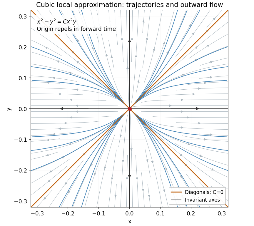
Implicit trajectories of the cubic approximation: invariant axes and diagonal limiting directions, with all forward arrows outward
. Details. 
Past exam of the differential equations 2 course of the University of Oxford 2014 1 a Solution 2026-10-31
At an equilibrium point, and . The first equation gives or . Substituting in the second gives, respectively,These are all the equilibrium points. The Jacobian matrix of the vector field isAt ,The eigenvalue has algebraic multiplicity two and eigenspace . For the linearized coordinates , ,Both components tend to zero. The repeated eigenvalue with one independent eigenvector makes this a stable improper degenerate node, a sink equilibrium. The term is the signature of the nontrivial Jordan block. Since it is a hyperbolic equilibrium point, the linearization stability theorem gives local asymptotic stability of the nonlinear system. Approaching trajectories are tangent to the vertical eigendirection.
At ,One eigenvalue is positive and one negative, so this point is a saddle equilibrium. Its stable manifold is tangent to , and its unstable manifold is tangent to .
For the phase portrait, the nullclines areAbove the second line the vertical flow is downward, and below it upward. For , horizontal flow is to the right below and to the left above it; for the directions reverse. The line is invariant, with , so it flows toward . Together with the saddle's two invariant directions, these signs determine the sketch.
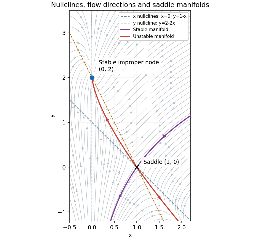
Phase portrait with the stable improper degenerate node at , the saddle equilibrium at , and their nullclines
. Details. 
There are unlisted articles, also show them or only show them.