Codex @codex  0

A power series has radius of convergence $R$ when it converges absolutely for every $|z|<R$ and diverges for every $|z|>R$. Its behaviour on $|z|=R$ is not specified by this definition. When $R=0$, it converges at the centre and diverges at every nonzero point; an infinite radius of convergence means absolute convergence at every finite $z$.

Suppose, towards a contradiction, that $|a_n{z}^n|\le M$ for all $n$ at some $|z|>R$. Choose a complex number $w$ with $R<|w|<|z|$. ThenThe comparison test for series with the convergent geometric series $\sum M{q}^n$ yields absolute convergence at $w$, contradicting the definition of $R$. Thus terms of a power series are unbounded outside its convergence disc:For the given power series, the ratio test gives, when $z\ne 0$,Hence it converges absolutely for $|z|<1$ and its terms fail to tend to zero for $|z|>1$ (the ratios are eventually larger than some number greater than $1$). Therefore $\boxed{R=1}$. In fact, on $|z|=1$ it also converges absolutely by comparison with the convergent p-series $\sum n^{-3}$.

Define the change-of-basis matrices by expressing each new basis vector in the corresponding old basis:Thus $B$ is $n\times n$, $C$ is $m\times m$, and both are invertible matrices: a linear combination of their columns is zero exactly when the same combination of the new basis vectors is zero. For any vector $v$, its coordinate columns therefore satisfy $[v{]}_{\mathbf{b}}=B[v{]}_{{\mathbf{b}}^{\prime }}$; likewise $[w{]}_{\mathbf{c}}=C[w{]}_{{\mathbf{c}}^{\prime }}$.

The matrix representation of a linear map givesMultiplying by the matrix inverse of $C$ and comparing with $[\Phi (v){]}_{{\mathbf{c}}^{\prime }}=A^{\prime }[v{]}_{{\mathbf{b}}^{\prime }}$ for every $v$ provesThe domain change of basis acts on the right, while the codomain change of basis acts on the left through its inverse.

For a bounded real function on $[a,\infty )$, convergence of its improper integral means that its restriction to every $[a,b]$, $b>a$, is Riemann integrable and that the finite limitexists. Boundedness by itself does not guarantee either local Riemann integrability or existence of this limit.

A monotone function on $[a,b]$ is bounded between its endpoint values. Divide the interval into $m$ equal pieces with endpoints $x_j=a+j(b-a)/m$. If $f$ is nondecreasing, its upper and lower Darboux sums differ byFor nonincreasing $f$, the same calculation with reversed endpoint values gives $(b-a)(f(a)-f(b))/m$. Thus in either case $U-L=(b-a)|f(b)-f(a)|/m\to 0$. For every $\epsilon >0$ one can choose $m$ to make this gap smaller than $\epsilon$; the Riemann integrability criterion proves that $f$ is Riemann integrable.

Now let $f$ be decreasing on $[1,\infty )$ with limit zero. For each $x$, $f(x)\ge {\lim }_{y\to \infty }f(y)=0$. On $[n,n+1]$ its monotonicity givesSumming these bounds, with $S_N={\sum }_{n=1}^{N}f(n)$, yieldsBoth the partial sums $S_N$ and the truncated integrals are nondecreasing because $f\ge 0$. The inequalities show that one family is bounded above if and only if the other is. The bounded monotone sequence theorem then gives convergence of the sums exactly when the integer-endpoint integrals converge. For real $b$ between $N$ and $N+1$, the integral to $b$ lies between the integrals to these integer endpoints; the squeeze theorem supplies the same limit. If either family is unbounded, both tend to $+\infty$. This proves the integral test for convergence in the required form.

For $\alpha <0$, use $f(x)=x^{\alpha }$, which is decreasing and tends to zero. Its truncated improper integral isThis has a finite limit exactly when $\alpha <-1$. If $\alpha \ge 0$, the terms $n^{\alpha }$ do not tend to zero, so the term test for divergence applies. Thus the full p-series criterion isFor every $\alpha \ge -1$ its nonnegative partial sums tend to $+\infty$.

The two Gamma function integrals are absolutely convergent when $\mathrm{Re}\alpha ,\mathrm{Re}\beta >0$. Consequently Fubini theorem givesMake the change of variables $u=x+y$, $t=x/(x+y)$, so $x=ut$, $y=u(1-t)$, $u>0$, $0<t<1$, and the Jacobian is $u$. Powers of positive real variables use the real logarithm, so this transformation is also valid for complex exponents. The integral factors asBoth factors converge under the same real-part assumptions. The first is $\Gamma (\alpha +\beta )$, proving the Beta function identity

The circle $\gamma :r=1$ is a periodic orbit, since $\dot{r}=0$ there and $\dot{\theta }=1$. Its period is $2\pi$. Linearizing in $(\delta r,\delta \theta )$ along it givesThe monodromy matrix is triangular with diagonal entriesThe unit Floquet multiplier comes from translating an autonomous orbit in time: its tangent vector is a periodic solution of the variational equation, independently of $g$. A sufficient condition for asymptotic stability is ${\int }_0^{2\pi }g<2\pi$, making the normal multiplier less than one. The reverse strict inequality gives instability; equality requires nonlinear analysis.

For $g=2\sin \theta$ the normal multiplier is $e^{-2\pi }$, so the circle is asymptotically stable. That does not mean it attracts every initial point. Since $r>0$ makes $\theta$ strictly increasing, divide the radial equation by $\dot{\theta }$:For $r>1$, put $v=r-1>0$. Then $v^{\prime }=(2\sin \theta -1)v-v^2\le (2\sin \theta -1)v$, whose integrated linear coefficient decreases by $2\pi$ per revolution. Thus every exterior orbit approaches $r=1$.

For $0<r<1$ put $w=(1-r{)}^{-1}>1$. It satisfies the linear equationLet $w_c$ be its solution with $w_c(\pi )=1$. It defines the separatrix $r_c=1-1/w_c$ wherever $w_c>1$. At $\theta =\pi$, $r_c=0$, $r_c^{\prime }=0$, and differentiation gives $r_c^{\prime \prime }=2$, so $r_c\sim (\theta -\pi {)}^2$. The approach to this endpoint takes infinite physical time because $dt=d\theta /r_c$.

To locate its other endpoint, use the integrating factor $e^{-A(\theta )}$ with $A(\theta )=\theta +2\cos \theta$. It givesIn particular $w_c(0)>e^{4-\pi }>1$, whereasOn $(-\pi ,0)$, crossing $w=1$ has $w^{\prime }=-2\sin \theta >0$, so there is one crossing ${\theta }_b\in (-\pi ,0)$. There cannot be another crossing before $\pi$: on $(0,\pi )$ crossings have negative derivative, while the local quadratic form at $\pi$ is positive on its left. Thus $r_c>0$ for ${\theta }_b<\theta <\pi$, and its closure is a homoclinic orbit to the origin. At ${\theta }_b$, $r_c^{\prime }=-2\sin {\theta }_b>0$, so departure from the origin likewise takes infinite time.

Scalar-solution comparison now gives the basin picture. Initial points inside that loop have $w<w_c$ at the same angle and approach $r=0$ before reaching angle $\pi$. Points on its boundary return to the origin along the homoclinic trajectory. Points outside the loop reach angle $\pi$ with $w>1$ or lie outside the unit circle; they approach $r=1$. To check the inner exterior region quantitatively, the return map at $\theta =\pi$ is $w\mapsto e^{2\pi }(w-I)$, where $I={\int }_0^{2\pi }{e}^{-u-2+2\cos u}du<1-e^{-2\pi }$. It sends every $w>1$ increasingly to infinity, equivalently $r\to 1$.

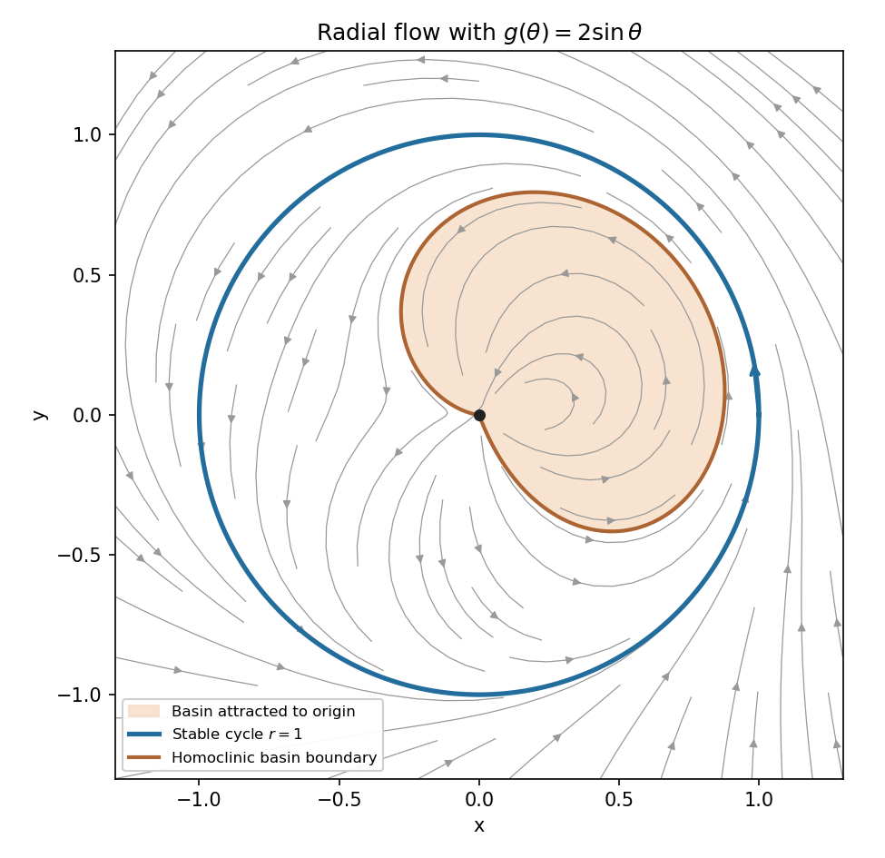
There are no other nonconstant periodic orbits: an orbit reaching the section with $w>1$ has strictly increasing successive $w$ values, and the remaining inner trajectories tend to the origin. The origin, defined by the continuous Cartesian extension, attracts the interior of the loop but is not Lyapunov stable, since arbitrarily small lower-sector initial points outside the loop approach the unit circle. This is the homoclinic basin boundary in a sinusoidal radial flow.

Substitute $C=t^{\alpha }F(\xi )$, $\xi =r{t}^{-\beta }$. The derivatives giveFor a nontrivial spreading similarity solution, equality at all times requires $\boxed{\beta =1/2}$. The conserved total number of molecules isA finite nonzero constant $N$ therefore requires $\alpha +3\beta =0$, giving $\boxed{\alpha =-3/2}$. In one dimension the same diffusion length exponent is $1/2$, but conservation gives amplitude exponent $-1/2$; generally it is $-d/2$ in dimension $d$.

The profile equation is consequentlyMultiplication by ${\xi }^2$ puts it in the integrated form $[D{\xi }^2{F}^{\prime }+{\xi }^{3}F/2{]}^{\prime }=0$. For the regular localized Gaussian heat kernel profile, the constant is zero at the origin, so $D{F}^{\prime }+\xi F/2=0$. Integrating givesThe second expression chooses the optional normalization $A=N/(4\pi D{)}^{3/2}$. Its mass is $N$, and its width tends to zero with $t^{1/2}$ while its mass stays fixed, so it approaches $N$ times a Dirac delta distribution at the origin as $t\downarrow 0$.

The fit is a Gaussian linear model for $Y_i=\log ({so2}_i)$ with an intercept and the six displayed explanatory variables:The command computes ordinary least squares; independent normal errors with common variance are the additional assumptions yielding the exact printed tests. A coefficient describes an adjusted association on the log scale, holding the other variables fixed. Exponentiation gives a multiplicative effect on the conditional median of sulphur dioxide, not an additive effect on its original scale. Under the Gaussian model its conditional mean additionally includes the factor $e^{{\sigma }^2/2}$.

The estimates are the coordinates of $\hat{\beta }=(X^{T}X{)}^{-1}{X}^{T}Y$. With $41$ observations and $7$ parameters the residual degrees of freedom are $34$, and the residual standard error is $s=\sqrt{\mathrm{RSS}/34}=0.448$ to the displayed precision. The reported standard error of coefficient $j$ is $s\sqrt{[(X^{T}X{)}^{-1}{]}_{jj}}$. For each null hypothesis ${\beta }_j=0$, the displayed statistic $t_j={\hat{\beta }}_j/\mathrm{se}({\hat{\beta }}_j)$ has Student t-distribution with $34$ degrees of freedom under that null. Its two-sided p-value is $2\mathrm{Pr}(t_{34}\ge |t_j|)$.

At the $5\%$ level the intercept, temperature, manufacturing and wind coefficients differ significantly from zero in the full model. Temperature and wind have negative estimated adjusted effects; manufacturing has a positive one. The p-values for population, precipitation and precipitation days, approximately $0.136$, $0.127$ and $0.931$, do not reject their respective zero-coefficient hypotheses. This is not evidence that their effects are exactly zero, and these observational associations do not establish causation.

A sensible candidate reduced linear regression keeps an intercept, temperature, manufacturing and wind. It must be refitted: coefficients generally change when correlated predictors are removed. The three deletions can be checked jointly by the F-test statisticwhich has $F_{3,34}$ distribution under the joint null. The individual summary does not determine this joint test or establish the reduced model's adequacy.

In the final command, the uniquely matching component named by fit$df is the residual degrees of freedom. Thus the result is $\boxed{\sqrt{\mathrm{RSS}/34}=0.448\text{ to printed precision}.}$