
The matrix sending the standard basis vectors to the given columns isWith the Hermitian inner product, the squared column norms are , , and . The off-diagonal products areThus the columns form an orthonormal basis, so and is a unitary matrix. Here the operation maps the old basis vectors to the new vectors; the inverse coordinate change of basis uses .
The Translation property of the Fourier transform givesFor the remaining integral, the same Translation property of the Fourier transform identifies as the Fourier transform of . By the product form of the convolution theorem, with inverse normalization ,But is supported in , whereas the four translated triangular functions making up are all supported in . Their product is identically zero. Therefore the requested integral is for every real .
The convolution is the length of the overlap of with . This overlap has length when and zero otherwise, so . The convolution theorem now givesThe value at zero is also the area of the triangular function, providing a normalization check on its Fourier transform.
Direct evaluation of the Fourier transform gives, for ,At the defining integral is the interval length, so . This also equals the continuous limit of the displayed formula.
Assume first that and are integrable functions, so that Fubini's theorem justifies changing the order of the two integrals. In the defining Fourier transform of the convolution, put :This proves the convolution theorem with the stated normalization:
For , split the Green's function integral at . Writing and givesFor , the two integrals areSubstitution and simplification yieldAt both contributions vanish. At the bracket is . The differential operator kills and sends to , so this also verifies the inhomogeneous equation.
The exceptional integer is , because then the integrals contain . In this caseand the Green's function integral becomesHere , and . Explicitly and . Thus both exceptional and nonexceptional formulas satisfy the required boundary conditions.
Choose the convention , where is the Dirac delta distribution, together with . The Green's function is continuous at and obeysThese conditions follow by integrating its differential equation across ; continuity prevents a derivative of the Dirac delta distribution. If and are homogeneous solutions satisfying the left and right boundary conditions, respectively, and is their Wronskian, thenFor take and . Their Wronskian is , and henceFor take and , giving andBoth formulas satisfy the endpoint conditions, continuity, and the unit jump directly. The unique solution of the boundary value problem isThe factor in the first formula matters: this Green's function is for the original monic differential operator, with ordinary measure , rather than for the operator multiplied by .
The homogeneous linear differential equation can be written in divergence form:One integration gives . Therefore the two cases areIn each case the displayed functions have linear independence throughout the interval. Imposing both homogeneous Dirichlet boundary conditions forces : for , , and for , . This also establishes uniqueness for the inhomogeneous boundary value problem.
The separation of variables solution with Dirichlet boundary conditions on the cuboid isThe constants are fixed by the initial density through Fourier sine series. The fastest term again has . When , its growth rate becomesThus the precise condition for no exponentially growing term isFor example, gives , while gives : either a sufficiently flat or a sufficiently elongated cuboid suppresses growth despite its unchanged volume. The function decreases to its minimum at , then increases without bound. Hence there are two positive threshold values, with growth only between them; equality leaves one stationary term and all other terms decaying.
The fastest temporal growth occurs for the lowest spatial eigenvalue, with . Its growth rate isFor a generic initial condition its coefficient is nonzero, so this term determines the long-time behavior. In fact, every nonzero, nonnegative initial density has , since the product of the three first sine eigenfunctions is strictly positive in the interior. ConsequentlyFor every term decays. At equality the first term is stationary and all higher terms decay: equality does not produce exponential growth. This is a reaction-diffusion equation threshold arising from competition between production and loss through the Dirichlet boundary condition.
For separation of variables, take and divide the reaction-diffusion equation by this product wherever it is nonzero:Each spatial term depends on a different variable and must be constant. Write and similarly for the other two factors. The Dirichlet boundary conditions give . A zero separation constant permits only a linear function and hence the zero solution; a positive value of likewise permits no nonzero function vanishing at both endpoints. The nontrivial choices are thereforeThe temporal ordinary differential equation isso, absorbing its constant multiplier into ,The superposition principle and completeness of the Fourier sine series give the stated threefold expansion with these factors. For an initial density , orthogonality also determines the constants:
It is enough to choose an admissible parameter, without solving the minimizing equation. Take in the Gaussian variational bound for an attractive Gaussian well. The Rayleigh-Ritz variational principle giveswhere an explicit remainder isThe denominator tends to as , proving in Big O notation. More precisely the binomial series givesand thereforeThis is an upper bound on the exact ground state energy, rather than an assertion that the leading coefficient of its exact weak-potential expansion is .
Differentiating the Gaussian variational bound for an attractive Gaussian well givesThus an interior stationary point obeysThe left side of the first equation increases strictly from zero to infinity, so there is exactly one such point. More explicitly,so is a strictly convex function on and is its global minimum. At that minimum the stationarity equation givesThere is a continuous limiting zero at , although at exactly is not a square-integrable function and hence is not an admissible trial. For a positive zero, division by and squaring gives , sois the unique positive zero. The other quadratic root is negative and inadmissible. Near zero,so the graph leaves the origin with slope , falls to its unique negative minimum, rises through , and grows as at infinity.
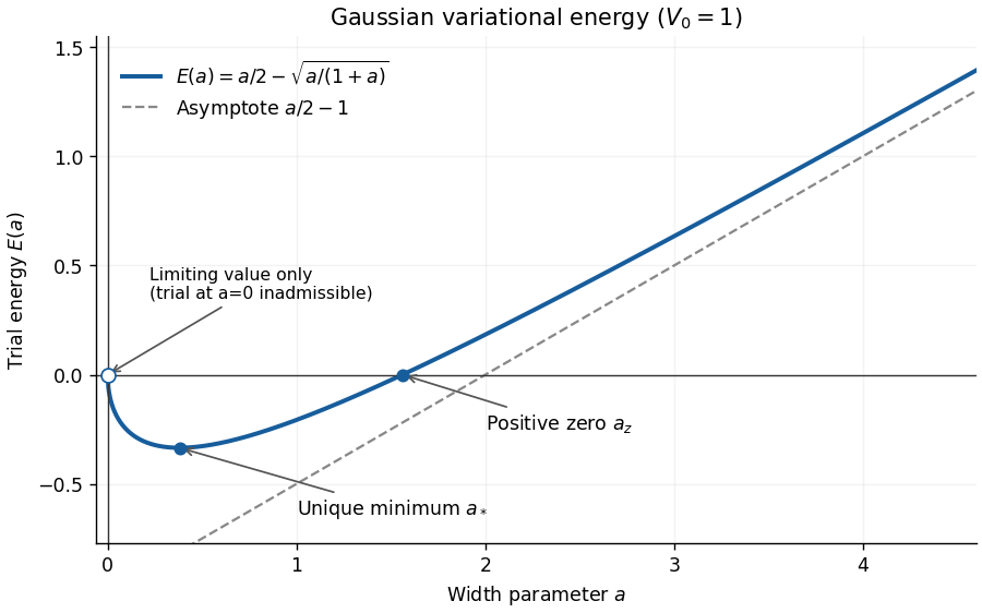
The Gaussian variational bound for an attractive Gaussian well at , showing its negative minimum and positive zero
. Details. 
By the Rayleigh-Ritz variational principle,Thus the attractive well supports a negative-energy bound state for every .
For the trial function, . The required Gaussian integrals areThe second formula follows by differentiating the first with respect to . Thereforeand division by gives the Gaussian variational bound for an attractive Gaussian well:This is a good trial family because it consists of smooth, positive, square-integrable functions decaying at both infinities. Each is an even function, matching the symmetry of the lowest bound state in this even potential, and the parameter varies its width. It also permits exact Gaussian integrals. Its Gaussian tail need not equal the exact exponential tail of a negative-energy bound state for the Rayleigh-Ritz variational principle to give a valid bound.
There are unlisted articles, also show them or only show them.