
Past exam of the mathematics course of the University of Cambridge 2008 iii Paper 50 1 Solution 2026-10-14
A phase diagram locates stable pure thermodynamic phases and their phase coexistence boundaries in a space of control parameters. For a concrete three-dimensional example, take the temperature, crystal-field parameter, and magnetic field of the Blume–Capel model. Its spins take values ; changing the cost of the zero-spin state can turn a continuous ordering transition into a discontinuous one. A local scalar description near the resulting tricritical point is the Landau-Ginzburg theoryThe three local control coordinates are , with varying linearly with the thermal scaling field. For , , the transition at is continuous. For , zero-field coexistence is at , and the magnetization jumps between zero and . The two loci meet at , the tricritical point.
The full three-dimensional phase diagram has an ordered coexistence sheet at , where the two opposite magnetizations exchange stability when changes sign. On its three-phase line it meets two nonzero-field tricritical wings. These wings are first-order phase transition surfaces between minima of the same sign but different magnitude, terminating at ordinary thermodynamic critical points. Their tricritical wing critical edges are found by :Indeed fixes , and substituting into and gives ; ensures a stable critical quartic minimum. The two signs give the two wings. All transition surfaces and critical edges end together at the tricritical point. The following plot uses ; its wing surfaces come from the exact tricritical wing coexistence factorization, rather than schematic unconstrained surfaces.
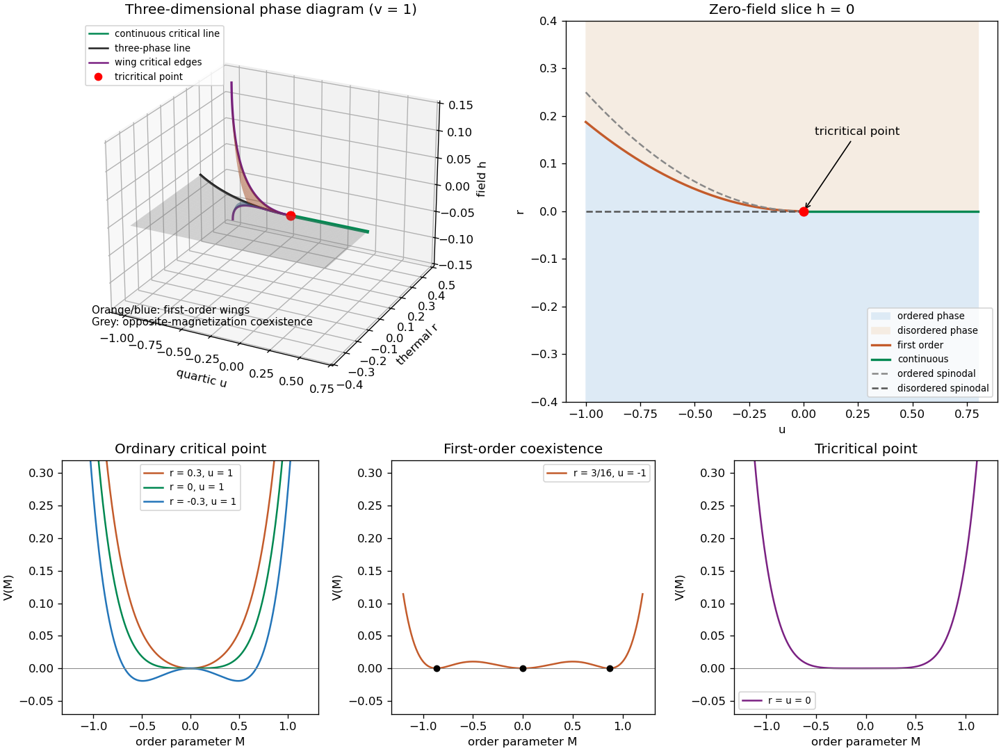
Tricritical coexistence surfaces, the zero-field phase diagram, and ordinary, first-order and tricritical Landau potentials
. Details. 
The unheaded requests for critical exponents follow from the uniform equation of stateFor an ordinary thermodynamic critical point, is fixed and , . At , , the small ordered minimum obeys , so the order-parameter critical exponent is . Above the transition , giving the magnetic-susceptibility critical exponent . At , , so the critical-isotherm exponent is . At the tuned tricritical point, , instead below the transition and on its critical isotherm, while the disordered susceptibility remains . ThereforeBelow the transition the inverse susceptibility is , giving in the ordinary limit and in the tricritical limit. Thus both sides give the same susceptibility power, with different amplitudes.
To derive the general Ginzburg criterion, tune away all lower even nonlinearities and let the leading stabilizer be , . The equation of state gives , and its curvature at the ordered saddle is , so . The fluctuations of the order parameter averaged over a correlation volume are estimated by its long-wavelength quadratic covariance:The integral has a fixed dimensionless upper limit after ; this is a coarse-volume fluctuation estimate, not the ultraviolet-dominated point variance. Consequently the multicritical Ginzburg ratio isThe Landau approximation is asymptotically controlled by this test only when the ratio tends to zero. This gives the upper critical dimensionThe same threshold follows by giving its Gaussian engineering dimension : the coupling to has scaling exponent , which becomes relevant below .
For , the fluctuation ratio diverges and the saddle calculation cannot predict the generic interacting critical exponents. At the test is marginal, not a proof of changed power exponents: the ratio has zero thermal power and marginal interactions can produce logarithmic corrections. Thus the PDF's inclusion of equality in a blanket claim about wrong power exponents needs this qualification. The Landau-Ginzburg theory as a fluctuating field theory remains useful; what loses validity is its fluctuation-free Landau approximation.
Past exam of the mathematics course of the University of Cambridge 2008 iii Paper 49 1 Solution 2026-10-14
For a finite-dimensional Lie algebra, write for its Adjoint representation. The Killing form is the symmetric bilinear formThe Jacobi identity gives . Using the cyclic property of the trace,Thus it is an invariant bilinear form on a Lie algebra. If , the adjoint matrix has entries . Its trace product yields the structure constants of a Lie algebra formulaA semisimple Lie algebra has zero solvable radical, equivalently no nonzero solvable ideal. In characteristic zero, the Cartan criterion for semisimplicity characterizes it by nondegeneracy of its Killing form. A real compact Lie algebra is the Lie algebra of a compact Lie group, equivalently one admitting a positive-definite invariant inner product. For a real semisimple algebra, the compactness criterion from the Killing form says compactness is equivalent to negative-definiteness of . An abelian compact-type algebra has zero Killing form, so this last characterization specifically concerns the semisimple case.
Past exam of the mathematics course of the University of Cambridge 2008 iii Paper 47 2 Solution 2026-10-14
Use the two-sided spectral density of a stationary process conventionThus white noise of variance has density .
Absolute summability makes the linear filter of a stationary time series well defined in : . Its mean is . For its autocovariance, continuity of the inner product givesThe sum is absolutely convergent because . It depends only on , proving weak stationarity. Inserting the spectral inversion formula and exchanging the absolutely dominated sum with the integral yieldsHere the coefficients are real, so the two factors are complex conjugates. This is the spectral density transformation under a linear filter.
Applying a second linear filter of a stationary time series givesThe composition of absolutely summable time-series filters can also be calculated directly:Indeed ; this bound also justifies the interchange of the two sums. The filter gain multiplies under this composition. The sketches for the two individual filters are:
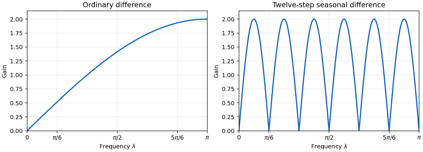
Ordinary and twelve-step seasonal difference-filter gains
. Details. 
Past exam of the mathematics course of the University of Cambridge 2008 iii Paper 46 4 Solution 2026-10-14
Let be the distinct observed event times, with individuals at risk just before and events there. Parameterize the event-time distribution by the conditional failure probabilities . Under independent censoring, the survival part of the nonparametric likelihood groups into factorsAn individual still under observation at contributes either a failure factor or a survival factor; later-censored individuals contribute the latter factors until censoring. Maximizing each factor independently gives , including the boundary solutions when or . Multiplying the conditional survival probabilities yields the Kaplan–Meier estimatorThe notation here denotes the survivor function, as in the question. The estimator is constant between event times. Under the usual simultaneous-event convention, individuals censored at remain in its risk set while events are processed, and are then removed.
There are unlisted articles, also show them or only show them.