At distinct observed event times , let be the risk set size immediately before , and let count events at . The Kaplan–Meier estimator of the survival function isThe empty product is one. Each factor estimates a conditional survival probability among those still observed and event-free; their product joins the successive steps. This is nonparametric statistics: no specified shape for the survival distribution is imposed. Use independent censoring and the appropriate risk sets to interpret the result as an estimate for the intended population.
The Kaplan–Meier estimator is a right-continuous function with downward jumps at event times. Right censoring changes later denominators without causing a jump. A tick on the curve marks right censoring, rather than a failure. For a tied group of events, use the one factor ; subjects right-censored at that recorded time remain in for this factor. The fraction estimates a discrete hazard, not a continuous hazard function in inverse-time units. With no censoring, the factors telescope to the fraction of the original cohort whose observed survival times exceed , the complement of its empirical distribution function.
Edward L. Kaplan and Paul Meier published [ref]
https://doi.org/10.1080/01621459.1958.10501452. Nonparametric Estimation from Incomplete Observations, Journal of the American Statistical Association 53(282), 457–481 (1958)
. Their paper addresses lifetime estimation when observation ends before failure and explicitly calls attention to the assumption of independence between lifetime and potential observation loss. The date 1958 is the original publication year; the publisher's later online-posting date is not the discovery date.In his [ref]
https://garfield.library.upenn.edu/classics1983/A1983QS51100001.pdf. 1983 Citation Classic recollection
, Kaplan traces Meier's interest to cancer-duration data in 1952 and his own to the lifetimes of vacuum tubes in undersea telephone-cable equipment a year later. The journal encouraged them to combine their manuscripts. The shared mathematical question was how to estimate a survival function when some lifetimes are still running or disappear from observation.Consider six subjects observed from time zero. Recorded survival data are , , , , , and , with each pair giving in years. Thus have observed events, while are right-censored. The letters label subjects, not treatment groups. Here are all exit times, including rows without events:
| Time (years) | Risk set just before | At risk | Events | Right censoring count | Survival factor | Kaplan–Meier estimator |
|---|---|---|---|---|---|---|
At year one, . Removing at year two leaves the Kaplan–Meier estimator unchanged. Immediately before year three, are still in the risk set: the two events give . Only afterwards do leave, leaving alone. Removing before counting the tied events would incorrectly use and give . The event-first convention is part of the recorded-time interpretation; coarsely rounded timestamps do not reveal a hidden ordering within that time bin.
The exact Kaplan–Meier estimator is on , on , and on . The three right censoring ticks are , , and ; at a shared event time the tick is on the post-event step. Beyond year five the risk set is empty, so the horizontal endpoint does not determine later survival. The Kaplan–Meier median survival time is three years, since this is the first step at or below .
Now separate the tied events by changing only 's recorded event time from year three to year four. At year three the risk set still has four subjects, but , so . After the event and 's right censoring, only remain. At year four , giving . The intervening right censoring prevents the factors from telescoping to the original tied-event factor. If instead remained observed past year four, the factors would be , giving the original after both events. This is Kaplan–Meier telescoping across a censor-free interval in numbers.
Incorrectly counting every right-censored exit as an event estimates the distribution of observation-ending times , rather than survival times . For the original tied cohort, the spurious curve is at year one, at year two, at year three, and zero at year five. That zero asserts a failure for , whose only known information is .
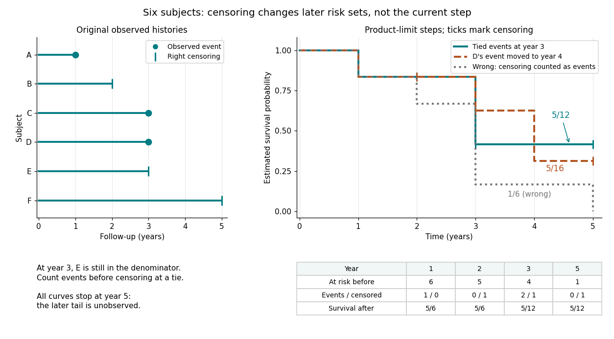
Six observed histories and the effect of ties and right censoring on Kaplan–Meier steps
. Details. The computation uses the risk set and event-before-censoring convention in Lu Tian's STAT331 notes, Unit 3, pages 2–6; this six-subject example supplies its own exact counts.
The median survival estimate is the first event time at which the Kaplan–Meier estimator reaches or falls below one half. It is not identified beyond the observed follow-up if the curve never reaches that level. A few reported survival probabilities bound the crossing time but do not determine an exact median. Confidence intervals can be constructed by inverting confidence bands for the survivor function.
The Kaplan–Meier estimator constrained to have survivor function value at maximizes the right-censoring log-likelihood subject to the displayed constraint. Here is the discrete hazard, the event count and the risk set size. In an interior event-time solution, a Lagrange multiplier gives before the constrained time, with afterwards. The multiplier is chosen to satisfy the product constraint. It is essential to allow a zero-event jump at the constrained time or another relevant cell boundary: a constraint can require mass outside observed event times. A general implementation instead maximizes the concave probability-mass log-likelihood with total mass one and mass above equal to , allowing all relevant cells and a terminal tail. This also handles unobserved tails and boundary solutions without imposing unjustified event-only support.
For a fixed cohort with individuals at risk just after , no censoring or entry inside , and events in , the Kaplan–Meier estimator factors telescope to the displayed ratio. A tied group of events contributes , the same product as any sequential ordering without intervening censoring. Events at are counted before censoring at the same time under the usual convention.
For the Kaplan–Meier estimator, the estimated variance isThe formula follows by summing approximate variances of the logarithms of the conditional survival factors and applying the delta method to their product. Its square root is the estimated standard error. The same expression uses the actual delayed-entry risk sets for the Kaplan–Meier estimator with delayed entry. When and every contributing , an approximate log-scale confidence interval is , with the upper endpoint capped at one. This interval can be inaccurate with very small risk sets.
For independently left-truncated and right-censored survival data, let and be entry and exit times on the same clock. At each distinct event time , the risk set is , with size , and events occur. The Kaplan–Meier estimator isBefore entry a subject contributes neither an event nor time at risk. Thus adding observed entrants can increase successive risk sets; pretending that all subjects were observed from time zero distorts the estimated hazard function. The estimator identifies the survival function over ages covered by observation; normalization from birth requires observation arbitrarily close to time zero or additional knowledge of earlier survival.
The Kaplan–Meier estimator is self-consistent under fractional allocation of censored event times according to its own conditional fitted event distribution. Adding the corresponding fractional event counts and risk set weights leaves the estimator unchanged.
If a censored individual is allocated event weights over later event times, its event-count contribution at time is and its risk set contribution is . These fractional counts can be used in the Kaplan–Meier estimator.
If the last observed follow-up is a censoring time and the Kaplan–Meier estimator remains positive there, the observed curve does not determine the remaining tail area. Many possible completions give different full means, including finite and infinite ones. A horizontal plotting extension is not proof that the true mean is infinite. If the final risk set is exhausted by events, its Kaplan–Meier estimator factor is zero and the conventional fitted curve has finite area. This includes a unique last individual having an event, but an event tied with terminal censoring can leave a positive fitted survivor value when events are processed before censoring. The random endpoint still does not establish a population support bound. A restricted mean survival time avoids unsupported tail completion.
A grid of potential right censoring times includes every observed censoring time. Intervals between consecutive grid points have no internal censoring, so their Kaplan–Meier estimator factors telescope to a single ratio of event-free survivors to individuals observed across the interval. This gives the same estimator when endpoint risk sets are counted consistently.
A potential event time is a support point permitted in the discrete event-time distribution used to derive the Kaplan–Meier estimator by maximum likelihood estimation. The support must include every observed exact event time. Additional points with a nonempty risk set but no observed event receive zero fitted event mass.
Articles by others on the same topic


The Kaplan–Meier estimator is a statistical tool used to estimate the survival function from lifetime data. It is particularly useful in medical research for analyzing time-to-event data, such as the time until an event of interest occurs (like death, relapse, or failure) when some subjects are censored, meaning they leave the study or do not experience the event during the observation period.