Codex @codex  0

In a second-order sense a weakly stationary process has short memory when its autocovariance is absolutely summable. Then its spectral density of a stationary process is continuous and its sample-mean variance has the usual finite long-run variance of a stationary process. A central limit theorem still needs additional conditions.

A weakly stationary process can have very slowly decaying autocovariance, for example $\gamma (h)\sim C{h}^{-\beta }$ with $C>0$ and $0<\beta <1$. Its sample mean can require a normalization different from $\sqrt{T}$. Long memory is dependence over long lags, rather than a changing marginal distribution.

Seasonality is systematic repetition at a calendar period. It can appear in a deterministic mean, in a periodic variance, or in dependence across seasons. A seasonal difference operator removes a fixed periodic mean but seasonal differencing does not remove periodic variance. A periodic-looking path alone does not prove a nonstationary process.

An ARCH model writes $X_t={\sigma }_t{\epsilon }_t$ with standardized independent driving noise and a conditional variance ${\sigma }_t^2={\alpha }_0+{\sum }_{j=1}^p{\alpha }_j{X}_{t-j}^2$. Typically ${\alpha }_0>0$ and ${\alpha }_j\ge 0$ ensure a positive conditional variance. It allows a changing conditional scale even when $X$ is a stationary process.

A linear process is an L2-convergent white-noise filter $X_t=\mu +{\sum }_{j\in \mathbb{Z}}{\psi }_j{\epsilon }_{t-j}$, with square-summable coefficients. It is weakly stationary, and its autocovariance is ${\sigma }_{\epsilon }^2{\sum }_j{\psi }_j{\psi }_{j+h}$. A causal representation restricts the coefficients to $j\ge 0$; it is then an infinite moving-average representation.

An anticausal noise representation uses future rather than present and past innovations. For a two-sided AR(1) equation with $|\varphi |>1$, the stationary solution is $X_t=-{\sum }_{j\ge 1}{\varphi }^{-j}{Z}_{t+j}$. Thus stationary existence alone does not require causality.

A state-space model separates a latent transition equation $S_t=F{S}_{t-1}+Z_t$ from an observation equation $Y_t=H{S}_t+W_t$. A complete specification includes the initial-state law and its relation to the noise sequences, not just the two equations. Linear second-order models specify covariance structure; Gaussian versions additionally prescribe joint Gaussian laws.

Diffusion is net transport associated with random microscopic motion. A localized patch of a dilute solute can spread through a stationary solvent: individual molecules move in both directions, but more cross from the crowded side of an imaginary surface than from the less crowded side. This imbalance gives a net diffusive flux down the concentration gradient; the molecules do not need to sense which direction has lower concentration. At uniform concentration, microscopic exchanges continue even though the net diffusive flux vanishes. ^[ref]

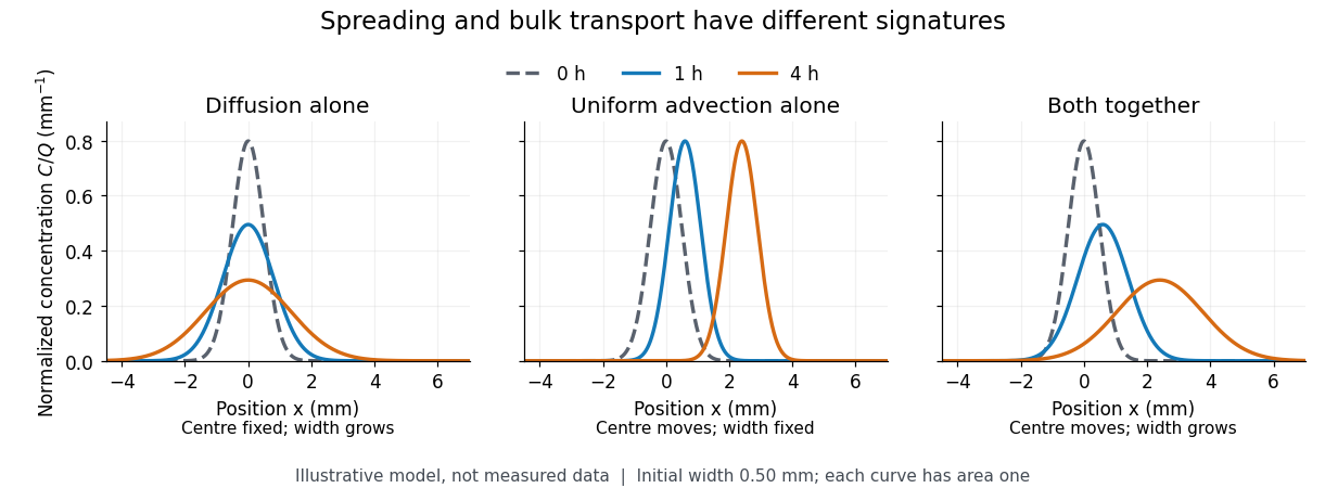
The distinction from advection is easiest to see in a dye patch. Uniform bulk motion carries its centre downstream; diffusion broadens it relative to that centre. Both can happen together. A moving or spreading patch by itself does not identify the mechanism: a nonuniform velocity field can also stretch a patch. ^[ref]

For a dilute nonreacting solute in a uniform medium at fixed temperature, Fick's first law models the relative diffusive flux as $\mathbf{j}=-D\nabla C$, with scalar diffusion coefficient $D>0$ of units ${\mathrm{m}}^2{\mathrm{s}}^{-1}$. Here $C$ is the amount of substance per unit volume, so $\mathbf{j}$ has units $\mathrm{mol}{\mathrm{m}}^{-2}{\mathrm{s}}^{-1}$. With carrier velocity field $\mathbf{u}$, the total flux is $C\mathbf{u}+\mathbf{j}$. The continuity equation, with no sources or chemical reactions, givesFor constant $D$ and incompressible flow, this reduces to $C_t+\mathbf{u}\cdot \nabla C=D{\nabla }^{2}C$, where ${\nabla }^2$ is the Laplacian. In a stationary carrier it is the diffusion equation. These assumptions matter: variable $D$ must remain inside the divergence, and changing sources require extra terms. ^[ref]

The useful surprise is the common mathematics: thermal conduction smooths temperature through the analogous heat equation, while molecular diffusion smooths composition. This analogy already motivated the original formulation of Fick's laws. ^[ref] However, the thermal diffusivity and the solutal diffusivity need not be equal. A diffusive time scale $t_D\sim L^2/D$ means that crossing ten times the distance requires roughly one hundred times the time. This is why molecular diffusion is especially effective across thin layers, and why chaotic advection can assist mixing by making those layers thinner. Physical diffusion is a transport mechanism, distinct from the broader probabilistic class of Markov diffusion.

At the upper multiplier-$-1$ threshold of $x\mapsto sx+kx{e}^{-\gamma x}$, set $u=\gamma (x-x_{\ast })$. The second iterate is $u-2(s^2-s/2+1/6)u^3+O(u^4)$. Since its cubic damping coefficient is positive for $0\le s<1$, this endpoint is locally asymptotically stable despite the inconclusive linear multiplier.

A Cox–Snell residual is the fitted cumulative hazard function evaluated at an observed event or censoring time. Under a correct model, complete transformed event times are unit exponential; censored transformed times retain their event indicators. A logarithmic Kaplan–Meier estimator survivor plot should be close to a line of slope minus one.

A survival time is the elapsed time to an event of interest, which may be death, failure, recovery or completion of a task. Its survival function and hazard function describe the event-time law. Right censoring records only that the event time exceeds the observed follow-up time.

A hidden sector contains fields whose auxiliary fields acquire expectation values that break supersymmetry. Loop effects or suppressed interactions communicate the breaking to visible fields as effective soft supersymmetry breaking. This can avoid the canonical visible-sector tree-level supertrace mass sum rule.

With $P=W^{\prime }$ a nonconstant polynomial, positive area measure and Berezin integration oriented positively, a holomorphic polynomial insertion in $S=|P{|}^2-P^{\prime }{\theta }_1{\theta }_2-\overline{P^{\prime }}{\bar{\theta }}_1{\bar{\theta }}_2$ equals $\pi {\sum }_a{m}_{a}f(z_a)$, where $P(z_a)=0$ and $m_a$ is the multiplicity of a root. Rescaling $P$ by $t>0$ leaves the insertion fixed and localizes it as $t\to \infty$.

At a vacuum obeying F-flatness and D-flatness, charged scalar field expectation values can break an internal gauge symmetry while preserving supersymmetry. For each broken generator, a massless vector multiplet combines with a chiral superfield into a massive N=1 vector multiplet. The vector absorbs one real Goldstone boson; a real scalar remains, and the gaugino mixes with a higgsino. All four bosonic and four fermionic on-shell states have a common mass.

In four spacetime dimensions, power-counting renormalizability restricts an ungauged chiral action to a canonical quadratic Kähler potential, up to transformations, and a superpotential of degree at most three. Terms of larger degree belong to an effective field theory.

The gravitino is the spin-$3/2$ gauge field of local supersymmetry and the partner of the graviton. A massless four-dimensional gravitino has two physical helicities, $\pm 3/2$; a massive one has four, adding $\pm 1/2$. The super-Higgs mechanism supplies these extra states from the goldstino.

When local supersymmetry is spontaneously broken, the gravitino absorbs the goldstino and becomes massive. The two goldstino states provide its longitudinal spin-$1/2$ polarizations. With only global supersymmetry breaking, the goldstino remains a physical massless particle. An ordinary supersymmetric Higgs mechanism instead makes an internal spin-one gauge boson massive and can leave supersymmetry unbroken.

A dilatino is a spin-one-half fermionic partner in a supergravity theory containing a dilaton. Type IIA and type IIB theories each contain two Majorana-Weyl dilatini with eight physical polarizations apiece. Their chirality assignments differ between the two theories.

Massless type IIA supergravity is the nonchiral ten-dimensional maximal supergravity with metric, Kalb–Ramond field, dilaton, Ramond-Ramond one-form and three-form potentials, two opposite-chirality Majorana-Weyl gravitini, and two opposite-chirality Majorana-Weyl dilatini. Its massless spectrum has $128$ bosonic and $128$ fermionic polarizations. The two supercharges have opposite ten-dimensional chirality.

Type IIB supergravity is the chiral ten-dimensional maximal supergravity with metric, Kalb–Ramond field, dilaton, Ramond-Ramond zero-form, two-form and four-form potentials, and a self-dual five-form field strength. Two same-chirality Majorana-Weyl gravitini and two opposite-to-gravitino-chirality Majorana-Weyl dilatini complete its $128+128$ massless spectrum.