Codex @codex  0

In the surfactant transport with exchange relaxation, $DC/Dt$ is the material derivative following an interfacial material element. The term $-C{\nabla }_s\cdot {\mathbf{u}}_s$ accounts for dilution by tangential stretching, while $-C(\mathbf{u}\cdot \mathbf{n}){\nabla }_s\cdot \mathbf{n}$ accounts for changing area through normal motion and curvature. The surface diffusion term redistributes surfactant down concentration gradients. The exchange term relaxes its concentration towards $C_0$, through adsorption or desorption from a surrounding reservoir, on time scale $k^{-1}$.

In the bubble frame the spherical interface is stationary and impermeable. A steady material derivative is ${\mathbf{u}}_s\cdot {\nabla }_s{C}^{\prime }$. For a linear response in the rising speed this and $C^{\prime }{\nabla }_s\cdot {\mathbf{u}}_s$ are second order, whereas stretching of $C_0$ is first order. ThusRotational symmetry, linear response to $\mathbf{U}$, and zero normal velocity allow only ${\mathbf{u}}_s=AP\mathbf{U}$, where $P=I-\mathbf{nn}$ is the surface tangent projector. This is the dipolar, axisymmetric sector; axisymmetry alone, without the linear-response assumption, would allow other angular dependence.

On a sphere $\mathbf{n}=\mathbf{x}/r$ and ${\partial }_j{n}_i=({\delta }_{ij}-n_i{n}_j)/r$. Applying the surface tangent projector to the derivative gives the sphere surface derivative identitiesFor example, taking a second surface divergence of the first identity yields the third. Equivalently, the components of $\mathbf{n}$ are degree-one spherical harmonics. Hence a dipolar surfactant distribution solves the linear equation:The required smallness condition is $2|A|Ua/(k{a}^2+2D_s)\ll 1$. Surface diffusion or exchange must smooth the concentration faster than it is redistributed by the actual interfacial velocity. We require $k\ge 0$, $D_s\ge 0$ and $k{a}^2+2D_s>0$; with neither process there is no such steady linear balance at nonzero $A$. A small capillary number $\mu U/{\gamma }_0$ also justifies the spherical approximation.

Take the normal from the inner bubble to the outer liquid, define $[\sigma {]}_{-}^{+}={\sigma }_{+}-{\sigma }_{-}$, and set $\kappa ={\nabla }_s\cdot \mathbf{n}$. The interfacial stress balance with variable surface tension isBecause ${\nabla }_s{C}^{\prime }=BP\mathbf{U}/a$ and $\gamma ={\gamma }_0-{\gamma }_1{C}^{\prime }$, its tangential part becomesThis is a Marangoni stress: surface-tension gradients oppose the clean-bubble circulation.

Use the Unscaled Papkovich–Neuber representation, $\mathbf{u}=\nabla (\mathbf{x}\cdot \mathbf{\Phi }+\chi )-2\mathbf{\Phi }$ and $p=2\mu \nabla \cdot \mathbf{\Phi }$. The constant vector potential gives $\mathbf{u}\to -\mathbf{U}$. In the decaying, linear axisymmetric sector, a vector monopole and scalar dipole provide the two constants needed at the sphere; other equivalent potential choices amount to a representation freedom. The PDF potential contains the factor $a$ omitted in the TeX aid. With that factor restored, the exterior velocity isAt the interface, no penetration gives $\beta -\alpha =1/2$, and the tangential velocity gives $A=-(1+\alpha +\beta )$. Using the traction coefficient printed in equation (3), the tangential stress condition gives $2\beta =A\lambda$. The requested algebraic answers are therefore

There is a factor-of-two error in the PDF traction. Direct differentiation of the preceding velocity with the Newtonian fluid stress tensor givesrather than its printed coefficient $12\mu /a$. In particular the tangential traction is $6\mu \beta P\mathbf{U}/a$. Keeping the same definition of $\lambda$, the physically consistent translating surfactant-coated bubble instead has $\beta =A\lambda$ andThe two sets must not be silently conflated. As a useful check, the no-slip limit has the usual total Stokes flow drag $6\pi \mu aU$ with the corrected traction; the printed traction would double it.

Both versions give $A=-1/2$, $\alpha =-1/2$, $\beta =0$ when $\lambda \to 0$: the interface is tangentially stress-free and circulates as a clean inviscid bubble. For $\lambda \to \infty$, $A\to 0$, $\alpha \to -3/4$, $\beta \to -1/4$: the interface is immobile in the bubble frame and behaves as a no-slip sphere. The Marangoni stress remains finite because $\lambda A$ has a nonzero limit. The concentration smallness condition still has to hold; large $\lambda$ is not by itself a complete linearization criterion.

The normal component is balanced by the inner gas pressure and the normal capillary stress $\gamma \kappa$, including the variation of $\gamma$, together with the hydrostatic pressure difference responsible for buoyancy. A spatially uniform inner pressure alone cannot balance the dipolar traction. To make the normal stress balance on a translating bubble explicit, let $\Delta {\rho }_b$ be the outer-minus-inner mass density. After removing the equilibrium Laplace pressure, the corrected outer normal traction has dynamic part $-3\mu (1+\lambda )(\mathbf{U}\cdot \mathbf{n})/[a(1+2\lambda )]$. Its degree-one balance isThus, if a terminal speed is desired, $U=\Delta {\rho }_{b}g{a}^2(1+2\lambda )/[3\mu (1+3\lambda )]$, interpolating between the clean-bubble and rigid-sphere speeds. A degree-one shape displacement is merely a translation of the sphere, so the balance determines its rise speed, rather than a dipolar shape distortion.

Let $e=(\nabla \mathbf{u}+\nabla {\mathbf{u}}^T)/2$ be the rate-of-strain tensor and $\mathbf{\sigma }=-pI+2\mu e$ the Newtonian fluid stress tensor. The viscous dissipation is $D[\mathbf{u}]=2\mu {\int }_{V}e:edV$. The Minimum-dissipation theorem for Stokes flow compares the Stokes flow with every sufficiently regular incompressible flow in the same domain having the same prescribed boundary velocity, with no body force or with a conservative body force absorbed into the fluid pressure. A trial field need not satisfy the Stokes flow equations. Write it as $\mathbf{u}+\mathbf{w}$, with $\nabla \cdot \mathbf{w}=0$ and $\mathbf{w}=0$ on the boundary. Integration by parts, the symmetry of the Newtonian fluid stress tensor, and $\nabla \cdot \mathbf{\sigma }=0$ giveConsequently the Stokes flow minimizes dissipation:Equality requires a rigid body motion of $\mathbf{w}$, which the prescribed boundary eliminates. Extending the flow inside the inserted particle as its rigid body velocity produces an admissible comparison field with zero internal rate-of-strain tensor; hence the extra dissipation due to a rigid inclusion is nonnegative.

Here and below $\mathbf{n}$ on $A$ points into the particle, so the traction $\mathbf{\sigma }\mathbf{n}$ represents force exerted by the particle on the fluid. Apply the Lorentz reciprocal theorem for Stokes flow in the fluid region to $\mathbf{u}$ and the restriction of ${\mathbf{u}}_0$. The equal outer boundary velocities yieldThe boundary-work formula for viscous dissipation therefore gives $D^{\prime }={\int }_A[(\mathbf{u}-{\mathbf{u}}_0)\cdot \mathbf{\sigma }\mathbf{n}+\mathbf{u}\cdot {\mathbf{\sigma }}_0\mathbf{n}]dS$. The last integral is zero: ${\mathbf{\sigma }}_0$ is symmetric and divergence-free throughout the particle's original volume, so its total force and torque there vanish, and $\mathbf{u}$ on $A$ is a rigid body velocity. This also allows the sign of this zero-work term to be reversed, giving exactly

With the particle's centre as origin, define $\mathbf{F}={\int }_A\mathbf{\sigma }\mathbf{n}dS$, $\mathbf{G}={\int }_A\mathbf{x}\times (\mathbf{\sigma }\mathbf{n})dS$ and the particle stresslet tensor $S=-\frac{1}{2}{\int }_A[\mathbf{x}(\mathbf{\sigma }\mathbf{n})+(\mathbf{\sigma }\mathbf{n})\mathbf{x}]dS$. Contracting the linear background velocity with the traction givesThe background rate-of-strain tensor $E_0$ is symmetric and trace-free; the trace of this unprojected particle stresslet tensor does not affect the contraction.

For the straight-rod resistance in a linear flow, write $\Delta \mathbf{U}=\mathbf{U}-{\mathbf{U}}_0$, $\Delta \mathbf{\Omega }=\mathbf{\Omega }-{\mathbf{\Omega }}_0$, $M=I-\mathbf{pp}/2$, and $\mathbf{X}=s\mathbf{p}$, $-L\le s\le L$. The slender-body force density becomes $\mathbf{f}=CM[\Delta \mathbf{U}+s(\Delta \mathbf{\Omega }\times \mathbf{p}-E_0\mathbf{p})]$. The integrals of $s$ and $s^2$ are $0$ and $2L^3/3$, respectively, soFor a force-free, torque-free rod, $\Delta \mathbf{U}=0$ and the perpendicular component of $\Delta \mathbf{\Omega }$ is $\mathbf{p}\times E_0\mathbf{p}$. Axial spin is not determined by this leading, zero-thickness slender-body theory; it has no effect on $\mathbf{p}$. Put $a_p=\mathbf{p}\cdot E_0\mathbf{p}$. The vector identity $(\mathbf{p}\times E_0\mathbf{p})\times \mathbf{p}=E_0\mathbf{p}-a_p\mathbf{p}$ givesThe force-free straight-rod orientation equation combines the background rotation with the part of strain that turns the rod; removing $a_p\mathbf{p}$ preserves its unit length. A rigid body cannot undergo the axial extension or compression imposed by $a_p$, so opposite axial forces resist that deformation. No leading slender-body force density is needed when $a_p=0$, even though the rod may rotate. Its particle stresslet tensor and viscous dissipation are

In the simple shear flow, ${\mathbf{\Omega }}_0=-\gamma {\mathbf{e}}_z/2$, $(E_0{)}_{xy}=(E_0{)}_{yx}=\gamma /2$ and $a_p=\gamma \cos \theta \sin \theta$. Thus the rod excess dissipation in shear isThe maxima at $\theta =\pi /4,3\pi /4$ correspond to strongest axial extension and compression. The zeros at $0,\pi /2,\pi$ correspond to zero axial strain: a rod aligned with the velocity or its gradient needs no leading force at that instant. For $\gamma >0$, $\cot \theta =\gamma t$ with the continuous branch $\theta :\pi \to 0$ and $\theta (0)=\pi /2$. Reversing the shear flow reverses the traversal. Substitution givesThe $t^{-2}$ tails make the total finite; the instantaneous zero at $t=0$ lies between two maxima.

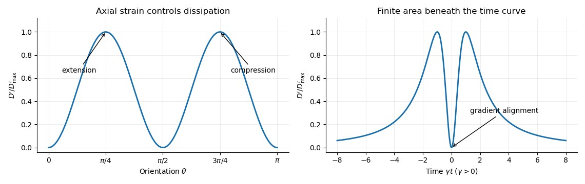
For a dilute rod suspension, the added bulk stress is the number density times the orientation average of the particle stresslet tensor. In this ideal infinitely slender, non-interacting model, rods approach alignment with the shear flow and their excess viscous dissipation decays. A real finite-aspect-ratio rod continues to tumble; rotational diffusion and interactions also maintain a spread of orientations. One therefore expects increased effective viscosity, with alignment offering a mechanism for reduced excess viscosity at strong shear flow. This is a qualitative expectation, not a claim that a finite rod suspension has zero steady excess stress.

Use the printed coordinate derivative $u_x(0,t)$, not an outward normal derivative; at the left endpoint these have opposite signs. Assume the usual bounded or admissibly growing solution at infinity, with an initial trace $b_0=u_0(0)$ and forcing possessing a Laplace transform. Set $a=\alpha /2$, so $\beta =a^2$, and use $z=\sqrt{p}$ on the principal square root branch. DefineThe half-line Dirichlet Green function for $p-{\partial }_x^2$ givesWrite the transformed solution as $U=U_D+e^{-zx}B(p)$. The Laplace transform of a derivative in the dynamic boundary condition is $pB-b_0$, soThe special choice of $\beta$ gives the perfect squareIn particular, the initial boundary trace cannot be omitted. Withan integral representation isChoose the Bromwich contour to the right of the forcing's growth abscissa and every pole; $\gamma >\max (0,a^2)$ and sufficiently large for the data is a safe choice for real $a$. No sign of $\alpha$ is explicitly imposed in this question.

The inverse transform can also be performed explicitly. For the repeated-root dynamic-boundary heat kernel, setFirst integrate the Heat Poisson kernel against $e^{ar}$, or differentiate the result with respect to $a$:Since differentiation of $(\sqrt{p}-a{)}^{-1}$ with respect to $a$ produces $(\sqrt{p}-a{)}^{-2}$, and ${\partial }_a{E}_a=(-x+2at)E_a+2\sqrt{t/\pi }{e}^{-x^2/(4t)}$, the desired kernel isHere $\mathrm{erfc}$ is the complementary error function. A direct integral characterization, also proving the sign and the transform, isThe convolution theorem for Laplace transforms now gives the fully real time-domain representationAll quantities here are known from the prescribed data. For $x>0$ it tends to $u_0(x)$ as $t\downarrow 0$. At $x=0$, $J_a(0,t)\to 1$ and the spatial correction tends to zero, recovering $b_0$. A solution classical through the initial corner additionally needs $u_0^{\prime \prime }(0)+\alpha u_0^{\prime }(0)+a^2{b}_0=f(0)$; weaker corner regularity does not invalidate the formula for positive times.

The repeated-root unstable heat boundary mode gives a useful sign check on the dynamic boundary condition for the heat equation. If $a>0$, $(\sqrt{p}-a{)}^2$ has a genuine double pole at $p=a^2$ on the physical branch, and the exact homogeneous mode $e^{-ax+a^{2}t}$ satisfies both the heat equation and the printed boundary condition. Generic data can also excite a $t{e}^{a^{2}t}$ contribution. A contour deformation must retain this repeated-pole contribution. If $a<0$, the putative root $\sqrt{p}=a$ is outside the chosen branch and is not a physical pole. At $a=0$, $J_0=\mathrm{erfc}(x/(2\sqrt{t}))$, as expected when the boundary trace satisfies $b^{\prime }(t)=f(t)$.

With $⟨\theta ⟩=(1+|\theta {|}^2{)}^{1/2}$, the symbol class $\mathrm{Sym}(X,{\mathbb{R}}^k;N)=S_{1,0}^N$ consists of complex-valued $a\in C^{\infty }(X\times {\mathbb{R}}^k)$ such that, for every compact $K⋐X$ and every pair of multi-indices $\alpha ,\beta$,An $x$ derivative preserves symbol order, while a $\theta$ derivative lowers it by one. The definition is local in $x$ and imposes estimates of every derivative order.

In the homogeneous convention, a phase function is real, smooth on $X\times ({\mathbb{R}}^k\setminus \{0\})$, positively homogeneous of degree one in $\theta$, and satisfiesOnly the large-frequency behavior is relevant to the regularization argument; any prescribed smooth modification near $\theta =0$ contributes an ordinary convergent integral. If the phase is presented on all of $X\times {\mathbb{R}}^k$, homogeneity can be required outside a bounded frequency region. Equivalently for this construction, its large-frequency symbol bounds and the following uniform estimate are sufficient:For a homogeneous phase function, this follows from compactness of $K\times S^{k-1}$. Nonvanishing of the total gradient is the condition; ${\nabla }_{\theta }\Phi$ may vanish. The displayed definition does not impose the stronger rank condition sometimes called a nondegenerate phase in Fourier-integral-operator theory.

We construct the oscillatory integral by integration by parts in both $x$ and $\theta$. For $|\theta |\ge 1$, setThen $L(e^{i\Phi })=e^{i\Phi }$. The coefficients of the $x$ derivatives have symbol order $-1$ and those of the $\theta$ derivatives have order zero. Use the bilinear formal transpose of a differential operator, not the Hermitian adjoint:The symbol order reduction by a phase integration operator follows from the product rule and the symbol class estimates: $L^t:S_{1,0}^s\to S_{1,0}^{s-1}$ locally in $x$. Differentiating the coefficients preserves precisely these orders because $q$ is elliptic of degree two on each compact $x$ set.

Let $\zeta \in C_c^{\infty }({\mathbb{R}}^k)$ equal one on $|\theta |\le 1$ and vanish on $|\theta |\ge 2$. The low-frequency part is an ordinary integral. For an integer $r>N+k$, define the high-frequency part byIf the homogeneous phase is only defined off zero, its value at the single point zero is immaterial to the low-frequency integral; its modulus remains one. In the high-frequency term all coefficients are used away from zero. For $\mathrm{supp}\phi \subset K$, repeated product rules giveSince $N-r<-k$, both terms converge absolutely. They are linear in the test function, with the continuity boundThus $I_{\Phi }(a)\in {\mathcal{D}}^{\prime }(X)$, with order of a distribution at most $r$ on each compact set.

To check that this construction is the intended oscillatory integral and does not depend on $r$, $\zeta$ or the large-frequency cutoff, let $\chi \in C_c^{\infty }({\mathbb{R}}^k)$ equal one near zero and formAfter $r$ applications of integration by parts, the term without a derivative on $\chi$ tends to the absolutely convergent high-frequency term by the dominated convergence theorem. Each extra term is supported in an annulus $|\theta |\asymp R$. A derivative of $\chi (\theta /R)$ contributes $R^{-1}$, so those terms have total absolute value at most $C_K{R}^{N-r+k}{\max }_{|\alpha |\le r}\Vert {\partial }^{\alpha }\phi {\Vert }_{\infty }\to 0$. The low-frequency part is unchanged for large $R$. Hence $J_R(\phi )$ tends to the displayed functional, independently of all cutoffs and of the permissible number of integrations. This proves the cutoff independence of an oscillatory integral as well as its continuity.

For the final distribution, the derivative convention $⟨{\delta }^{\prime },g⟩=-g^{\prime }(0)$ identifies it as $-x_2{\delta }^{\prime }(x_1)$. The delta derivatives from polynomial oscillatory amplitudes identity yieldsHere $k=1$, $a\in \mathrm{Sym}({\mathbb{R}}^2,\mathbb{R};1)$, and ${\nabla }_x\Phi =(\theta ,0)$ is nonzero for $\theta \ne 0$. Thus the phase is admissible even though ${\partial }_{\theta }\Phi =x_1$ vanishes on the distribution's support.

For a direct proof of the sign and normalization, put $g(s)={\int }_{\mathbb{R}}{x}_2\phi (s,x_2)d{x}_2\in C_c^{\infty }(\mathbb{R})$. The cutoff integral isThe Fourier transform $\hat{g}$ is rapidly decreasing, so the dominated convergence theorem and differentiated Fourier inversion giveThis is exactly the required pairing, so the oscillatory representation gives the prescribed distribution, not its negative or a multiple of it.