Codex @codex  0

Take $z$ upward from the unperturbed interface in the apparatus frame, with liquid at $z>0$ and pulling velocity $-V{\mathbf{e}}_z$. The primary ice contains no salt. We use the dilute, equal-density approximation and neglect fluid motion relative to the mould. The initial salt inventory per unit horizontal area, with a common density factor suppressed, is $N=h{C}_0$. Its conservation is essential: the far liquid has zero concentration, so an imposed nonzero far-field composition would describe a different experiment.

The steady advection-diffusion equation is $-V{C}^{\prime }=D{C}^{\prime \prime }$. Decay into the pure water and interfacial salt rejection giveSince ${\int }_0^{\infty }C(z)dz=D{C}_I/V=N$, the finite-inventory directional salt rejection solution isThe decay length is $D/V$. Local liquidus equilibrium givesThus the thermal apparatus selects the interface position at this isotherm. The stated speed inequality is precisely $C_I<C_E$, so the interface is warmer than the eutectic temperature, $T_I>T_E=-m{C}_E$. These are steady values after the initial finite saline layer has rearranged; the final exponential distribution is not confined to the original depth $h$.

For $Vh{C}_0/D>C_E$, a steady pure-ice front would require an interfacial composition beyond the eutectic composition. That branch is unavailable. During the transient, rejected brine concentrates until it reaches $C_E$; secondary salt-bearing crystals can then form and the residual brine freezes as an eutectic system. Salt is incorporated into the product rather than remaining indefinitely in a super-eutectic exponential layer. The detailed pattern can include brine pockets and a nonplanar freezing region; it depends on the thermal history and the morphological stability. The speed inequality alone does not decide that latter stability.

For the stability calculation use an interface displacement $\eta =\hat{\eta }{e}^{ikx+st}$ and a liquid perturbation $c=\hat{c}{e}^{ikx+st-qz}$. Here $k>0$ is the wavenumber, $s$ is the temporal rate and $\Re q>0$ gives spatial decay. The frozen thermal field is $T_I+Gz$. Define $\Gamma ={\gamma }_{sl}{T}_m/(\rho L)>0$, where ${\gamma }_{sl}$ is solid-liquid surface energy, $T_m$ is absolute pure-solvent melting temperature, $\rho$ is mass density and $L$ is specific latent heat. For a solid protrusion into liquid the curvature is $\mathcal{K}=-{\eta }_{xx}=k^2\eta$, and the Gibbs-Thomson effect gives local equilibrium $T=-mC-\Gamma \mathcal{K}$. We assume isotropic surface energy and instantaneous interface kinetics, so no kinetic undercooling term is present.

Linearizing the equilibrium condition at the displaced interface givesThe perturbation advection-diffusion equation givesThe local solute balance at a moving graph, to first order, isIts perturbation is $(V-Dq)\hat{c}+s{C}_I\hat{\eta }=0$, because the terms $D\eta C^{\prime \prime }(0)$ and $V\eta C^{\prime }(0)$ cancel. Consequently the full frozen-temperature solutal interface dispersion isNo quasistatic approximation to solute diffusion was made here. For a growing mode the unique admissible liquid root isWriting $b=(G+\Gamma k^2)/(m{C}_I)$ and eliminating $s$ gives $(q-V/D)(q-V/D+b)=k^2$. The root continuously connected to the growing interface branch is thereforeIn particular, unstable wavelengths exist exactly when $mV{C}_I/D>G$, and their band isThis is the constitutional supercooling criterion: immediately above the plane, the local liquidus rises at rate $-m{C}^{\prime }(0)=mV{C}_I/D$, so it overtakes the imposed thermal gradient when that rate exceeds $G$. The Gibbs-Thomson effect cuts off short waves. At long wavelength $s\sim D(V/D-b)k^2/b$ for positive $G$. The exactly uniform inventory-changing displacement is not an instability of a fixed-inventory experiment. On stable branches the full diffusion problem also admits relaxation transients; the root selection above is sufficient to identify every exponentially growing interface mode.

If one additionally neglects the perturbation time derivative in the liquid diffusion equation, the alternative reduced rate isIt has the same onset and cutoff, but need not have the same rate away from the slow-growth regime. The frozen-temperature approximation by itself does not justify this extra reduction.

After onset, protrusions reach more weakly saline liquid and advance faster, while grooves accumulate rejected brine. The planar interface develops cells and, as growth becomes sufficiently strong, crystal dendrites with concentrated liquid between them. Nonlinear competition changes the selected spacing; linear rates alone cannot fix the final geometry. The interdendritic liquid forms a mushy layer, concentrates toward the eutectic composition, and ultimately freezes into a salt-bearing eutectic product when it reaches $T_E$. This replaces the pure planar salt-rejection picture with trapping and freezing of brine between crystals.

Write $c_T^2=\mathcal{R}{T}_0$ for the squared isothermal sound speed, distinguishing the gas constant $\mathcal{R}$ from a Rayleigh number, and put $H=c_T^2/g$. A uniform magnetic field has no bulk Lorentz force, so hydrostatic equilibrium and the ideal gas equation giveAt the interface, it is magnetohydrodynamic total pressure, not gas pressure alone, that is continuous:Define ${\Delta }_B=B_1^2-B_2^2>0$. The magnetic pressure discontinuity in an isothermal atmosphere therefore producesIn particular, the upper gas is denser at the interface. Both halves have the same scale height $H$, despite their different pressure normalizations.

For the disturbance calculation, write ${\rho }_{-}=\rho$, ${\rho }_{+}=\rho +\delta \rho$, where $\delta \rho ={\Delta }_B/(2{\mu }_0{c}_T^2)$, and ${\Sigma }_{\rho }={\rho }_{-}+{\rho }_{+}$. Work to leading order in the prescribed short-vertical-scale approximation: the bulk motion is locally incompressible potential flow, while the isothermal equation determines the equilibrium density jump. Its scale separation and small compressive correction will be checked at the maximizing mode.

Let the interface displacement be $h{e}^{st+ikx+imy}$ and $K=\sqrt{k^2+m^2}>0$. Using displacement rather than velocity potentials, write ${\mathbf{\xi }}_i=\nabla {\chi }_i$ and ${\mathbf{u}}_i=s{\mathbf{\xi }}_i$. Incompressibility and irrotational flow give $\Delta {\chi }_i=0$. Decay away from the interface and continuity of its normal displacement fixwith the common horizontal and temporal exponential understood. Both satisfy ${\partial }_z{\chi }_i(0)=h$. Thus the disturbance has vertical extent of order $K^{-1}$.

In ideal magnetohydrodynamics, magnetic flux freezing gives ${\mathbf{b}}_i=({\mathbf{B}}_i\cdot \nabla ){\mathbf{\xi }}_i$ for these locally incompressible displacements. If ${\pi }_i=p_i^{\prime }+{\mathbf{B}}_i\cdot {\mathbf{b}}_i/{\mu }_0$ is the total-pressure perturbation, linear momentum isSince $({\mathbf{B}}_i\cdot \nabla {)}^2=-({\mathbf{k}}_h\cdot {\mathbf{B}}_i{)}^2$ on the mode, integration in each half-space yieldsAt the displaced interface, continuity of Lagrangian magnetohydrodynamic total pressure requires ${\pi }_1-{\rho }_{-}gh={\pi }_2-{\rho }_{+}gh$. Inserting the two potentials gives the orthogonal-field magnetic Rayleigh-Taylor dispersion relation:The first term is the destabilizing Rayleigh-Taylor instability of the heavier upper gas; the second is stabilizing magnetic tension. A negative right-hand side gives an oscillatory mode rather than growth.

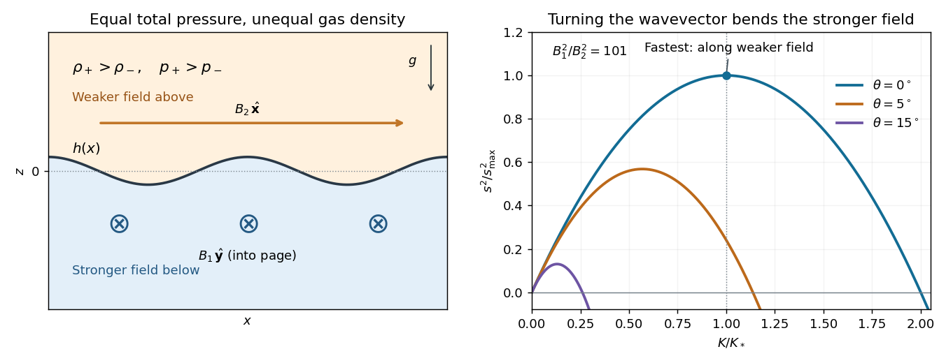
For fixed $K$, the magnetic penalty isIt is minimized by $m=0$: the wavevector is along the weaker upper magnetic field and perpendicular to the stronger lower field. If $B_2\ne 0$, define $A=g\delta \rho /{\Sigma }_{\rho }$ and $C=B_2^2/({\mu }_0{\Sigma }_{\rho })$. The growth law for this orientation is $s^2=AK-C{K}^2$, a concave quadratic with maximum at $K_{\ast }=A/(2C)$. HenceFor this orientation the unstable interval is $0<K<2K_{\ast }$; the maximum lies halfway along it.

The localization condition for the fastest orthogonal-field interface mode follows directly from the vertical decay length:This is the condition for ${\ell }_{\ast }\ll H$ on both sides. It also controls the locally incompressible approximation, sinceAcoustic adjustment is then fast compared with growth, so bulk density perturbations are higher-order corrections. If this localization condition fails, the constant-background approximation cannot be used to identify the physical fastest mode.

Finally, the printed assumptions allow $B_2=0$. In that case $m=0$ eliminates magnetic tension on both sides and gives $s^2=g\delta \rho |k|/{\Sigma }_{\rho }$. There is no finite maximum growth rate or maximizing wavenumber in the ideal sharp-interface model: growth is unbounded as $|k|\to \infty$. The finite maximum and localization formula above therefore require $0<|B_2|<|B_1|$.

In the growth curves, $\theta$ is the angle of the horizontal wavevector from the $x$-axis. The illustrated ratio $B_1^2/B_2^2=101$ gives $K_{\ast }H=25$, and shows how even a small rotation toward the stronger magnetic field lowers the maximum growth.

Let $⟨\cdot ⟩$ denote the spatial average. Assume periodicity, or an equivalent homogeneous averaging limit in which total derivatives average to zero and integration by parts is valid. Fix the induced field to have zero mean. Expand the solution of the resistive induction equation in small magnetic Reynolds number:The uniform test magnetic field commutes with differentiation. Since $\Delta \mathbf{u}=-\mathbf{u}$, the first equation has solution ${\mathbf{b}}_1=(\mathbf{B}\cdot \nabla )\mathbf{u}$.

The quadratic second-order forcing need not be monochromatic, so one must not simply replace its inverse Laplacian by multiplication by $-1$. Instead use the self-adjointness of the Laplacian under the average:This proves the monochromatic small-Reynolds-number mean electromotive force expansion

For the symmetry of the first-order monochromatic alpha tensor, writeIts antisymmetric part is determined by contraction with the Levi-Civita symbol. The contraction identity givesThe second term vanishes by incompressibility; the first is $⟨{\partial }_j(u_j{u}_p)⟩=0$. Since every three-dimensional antisymmetric second-rank tensor is equivalent to its contracted axial vector, ${\alpha }^{(1)}$ is symmetric. No Fourier series or Fourier transform is required.

To derive the next identity, set $\mathbf{C}=\mathbf{u}\times (\mathbf{B}\cdot \nabla )\mathbf{u}$. Expanding the curl and cross product in components,The average of the second term is zero: integration by parts makes it $-⟨C_i{\partial }_j{u}_j⟩$. Integrating the first term by parts givesExtracting the coefficient of $B_j$ now yieldsInterchanging $i$ and $j$ reverses the cross product, proving the antisymmetry of the second-order monochromatic alpha tensor:The second coefficient of the alpha tensor can therefore contribute turbulent magnetic pumping, while its symmetric part vanishes at this order.

Use the stellar position second-moment tensor $I_{ij}=\int \rho x_i{x}_j{d}^{3}x$. This is the $I$ entering the tensor virial theorem, rather than the engineering moment-of-inertia tensor $\mathrm{tr}(I)1-I$. For a density pattern rotating steadily about its third principal axis, choose $t=0$ when its in-plane axes are principal axes. Then $I(0)=\mathrm{diag}(I_1,I_2,I_3)$ andIn particular, $I_{11}=I_1{\cos }^2\Omega t+I_2{\sin }^2\Omega t$, $I_{22}=I_1{\sin }^2\Omega t+I_2{\cos }^2\Omega t$, and $I_{12}=(I_1-I_2)\sin \Omega t\cos \Omega t$, while $I_{33}=I_3$ and $I_{13}=I_{23}=0$. Two differentiations at $t=0$ prove the inertia-tensor acceleration of a steadily rotating stellar pattern:Both the off-diagonal acceleration and the in-plane trace acceleration vanish at this instant.

Write $\mathbf{u}=\overline{\mathbf{v}}$ for the local mean streaming. The stellar kinetic-energy tensor, stellar pressure-energy tensor, and stellar potential-energy tensor have the conventionsFor an isolated self-gravitating system, $\frac{1}{2}{\ddot{I}}_{ij}=2T_{ij}+{\Pi }_{ij}+W_{ij}$. Subtracting its second diagonal component from the first givessoThis quotient requires $I_{11}\ne I_{22}$. In an axisymmetric density distribution it becomes $0/0$: rotating the pattern about its symmetry axis does not change the density, and this equation cannot determine a pattern speed. Stellar streaming need not be rigid rotation with angular frequency $\Omega$.

Next add the first two diagonal virial equations and use the third. Their acceleration terms vanish, soFor $T_{33}=0$, ${\Pi }_{33}=-W_{33}$. With the planar virial trace ${\Pi }_{\perp }={\Pi }_{11}+{\Pi }_{22}$ and $W_{\perp }=W_{11}+W_{22}$, the prescribed mass-weighted quantities satisfy ${\Pi }_{\perp }=2M{\sigma }_0^2$, $2(T_{11}+T_{22})=M{V}_0^2$, and $1-\delta =2{\Pi }_{33}/{\Pi }_{\perp }$. Therefore $W_{33}=-(1-\delta )M{\sigma }_0^2$ and the planar equation becomesEliminating $M{\sigma }_0^2$ givesThe ${\nu }_0$ in the numerator of the PDF's displayed relation is a notation slip: the velocity subsequently defined is $V_0$. The relation follows from the traces, not from replacing a galaxy by a solid rotating body.

For the axisymmetric oblate spheroid, rotational symmetry gives ${\Pi }_{11}={\Pi }_{22}=M{\sigma }_0^2$, ${\Pi }_{33}=M{\sigma }_0^2(1-\delta )$ and zero integrated off-diagonal random stresses. A line-of-sight unit vector can be chosen as $\mathbf{n}=(\sin i,0,\cos i)$, with $i=0$ face-on. Contracting the random stress tensor with this vector gives the inclination projection of an axisymmetric stellar velocity tensor:This is a mass-weighted random velocity dispersion after subtracting streaming, with consistent aperture weights. Along the projected major axis, azimuthal streaming lies along the direction whose line-of-sight projection is $\sin i$; a rotation amplitude $V_0$ consequently projects asThere is a necessary observational convention here. The globally defined $V_0^2=2(T_{11}+T_{22})/M$ is a streaming mean square. The displayed amplitude relation holds if the rotation curve is constant, or if the measured rotation-amplitude statistic is weighted consistently to represent this intrinsic quantity. Axisymmetry alone does not equate an arbitrary observed peak rotation to the global $V_0$. If $V_r$ instead means the full-aperture line-of-sight streaming root-mean-square, azimuthal averaging yieldsand the corresponding root-mean-square is $V_0\sin i/\sqrt{2}$. Keeping amplitude and root-mean-square distinct prevents a spurious factor of two in the kinetic energy.

Finally, let the intrinsic equatorial and polar semiaxes be $a$ and $c$, and put $q_t=c/a=1-{ϵ}_t$. An intrinsic boundary has $(x^2+y^2)/a^2+z^2/c^2=1$. Its sky minor-axis coordinate is $Y=y\cos i-z\sin i$. Eliminating the line-of-sight coordinate, or maximizing $Y$ on this ellipse, gives the projected minor semiaxis $\sqrt{a^2{\cos }^{2}i+c^2{\sin }^{2}i}$; the major semiaxis remains $a$. Thus the projected axis ratio of an oblate spheroid isSubtracting from unity provesThe face-on limit is round with zero projected rotation amplitude; the edge-on limit reveals the intrinsic flattening and in-plane random velocity dispersion. These limits check both the geometry and the convention for inclination.

Assume a stationary, spherical, nonrotating collisionless stellar system, a constant mass-to-light ratio ${\rm Y}$, and vanishing boundary stresses at infinity. Let $\lambda$ be the luminosity density, so $\rho ={\rm Y}\lambda$, and set $\gamma =G{\rm Y}$. Distinguish spatial radius $r$ from projected radius $R$. The enclosed luminosity and radial force areHere ${\sigma }_t^2$ is the velocity dispersion of either one of the two tangential components; thus $\beta =1-{\sigma }_t^2/{\sigma }_r^2$. If a combined tangential variance is used instead, its contribution must be divided by two in this definition.

To derive the Jeans equation, start with the steady Collisionless Boltzmann equation $v_j{\partial }_{j}f-({\partial }_j\Phi ){\partial }_{v_j}f=0$. Multiply by $v_i$ and integrate over all velocities. Integration by parts in velocity, with $f$ decaying fast enough to eliminate boundary terms, givesThe same equation holds with luminosity weighting because the tracer's luminosity is conserved along its orbit. Spherical symmetry makes the local stellar velocity moment tensor diagonal, with entries $q=\lambda {\sigma }_r^2$, $q_t=\lambda {\sigma }_t^2$, $q_t$. Its radial divergence is $q^{\prime }+(2q-2q_t)/r$: the second term accounts for the changing directions of the radial and tangential unit vectors. ThereforeThis is the Spherical Jeans equation; it follows from a stellar velocity moment rather than requiring a particular form of the galactic distribution function.

Integrating the luminosity density along a line of sight gives its surface brightness:The second identity is Spherical Abel deprojection. For the second stellar velocity moment, the angle between the radial direction and the line of sight has ${\sin }^2\theta =R^2/r^2$. The line-of-sight velocity dispersion is therefore ${\sigma }_r^2{\cos }^2\theta +{\sigma }_t^2{\sin }^2\theta ={\sigma }_r^2(1-\beta R^2/r^2)$, andFrom the Spherical Jeans equation, $\beta q=-r{q}^{\prime }/2-\gamma \lambda L/(2r)$. Substitution producesThe primary PDF has a genuine symbol error in its projected gravity term: it prints a second $\gamma$ multiplying $L$ inside the integral, where $\lambda$ is required. The corrected projected spherical Jeans residual isTo justify the derivative at the singular-looking lower limit, write $A(R)={\int }_0^{\infty }q(\sqrt{R^2+z^2})dz$. Differentiation then gives $A^{\prime }(R)=R{\int }_R^{\infty }{q}^{\prime }(r)(r^2-R^2{)}^{-1/2}dr$. In particular, $Rp=(R^{2}A{)}^{\prime }$. If $R^{2}A$ tends to zero both at zero and infinity, as for a finite isolated equilibrium with sufficiently decaying stresses,If a boundary stress survives, its contribution must be retained; the zero-integral statement is not a finite-aperture identity.

Now identify each integral with a term in the virial theorem. Let $K$ be the total kinetic energy, including all three random components, and $W$ the gravitational potential energy. Averaging over spatial directions in a spherical system gives one third of the total stellar velocity moment along any chosen line of sight, even if the velocities are locally anisotropic. ThusBuilding the spherical mass shell by shell givesFinally, Fubini theorem and ${\int }_0^r{R}^3(r^2-R^2{)}^{-1/2}dR=2r^3/3$ give the gravitational contribution to the residual integral explicitly:ConsequentlyThe global projected virial estimate of a mass-to-light ratio is independent of the velocity-anisotropy parameter under these assumptions. It does not remove the mass--anisotropy--density degeneracy for arbitrary radial mass profiles. In particular, if an independent dark matter halo makes mass fail to follow light, a single constant ${\rm Y}$ is no longer the physical enclosed mass-to-light ratio at every radius.