
Past exam of the mathematics course of the University of Cambridge 2016 iii Paper 334 4 Solution Created 2026-10-03 Updated 2026-10-14
Use the same resistive-force theory convention as before: the force density is the fluid's force on the filament. Let be the usual cylindrical azimuth. Choose the orientation of a left-handed helix so that, as increases, decreases. With , ,Reversing the orientation of the tangent leaves the local drag tensor unchanged. Define . From resistive-force theory, the relevant force-density components areThese scalar axial and azimuthal components are uniform along the helix. Integration over its contour length , and use of the axial torque density , give the axial resistance matrix of a slender helix:Thus , as also required by the Lorentz reciprocal theorem. The signs here belong to , with forces and moments on the helix. The handedness reversal of helical hydrodynamic resistance reverses but leaves unchanged. If the positive rotation direction or handedness convention is reversed, the coupling sign reverses with it.
As a check on physical admissibility, the determinant of helical resistance in resistive-force theory isTogether with , this makes the hydrodynamic resistance matrix positive definite and the viscous power loss positive. Isotropic local drag would have , so rotating a helix would not propel it in this approximation.
For the pair, use a local additive resistive-force theory model: both helices have the same drag coefficients, and inter-helix hydrodynamic interactions and unresolved end effects are omitted. The right-handed helix has resistance entries . Define the signed motor motion byThe printed relative rotation specifies a magnitude rather than which helix rotates relative to which. Choosing instead reverses all signed speeds below.
The common translation speed and zero total force and torque obeyInternal motor forces and torques cancel in these totals. IntroduceSolving the three linear equations yields the opposite-handed counterrotating helical swimmer:For , and , , so , and . The opposite-handed helices counterrotate but contribute thrust in the same axial direction. The formula satisfies the specified relative rotation without identifying either laboratory rotation rate with the motor rate.
At , the second helix supplies no hydrodynamic resistance. The remaining helix must have , and invertibility of its hydrodynamic resistance matrix forces . Formally is the rotation of a zero-resistance motor shaft or vanishing second rotor; there is no physical finite second helix to propel or to provide a reaction torque. This is the vanishing reaction rotor in a helical swimmer.
At , equal-length opposite-handed helices haveThe translation-generated axial torques cancel between the two helices, and equal counterrotation balances the rotational torques. Their propulsive forces add, rather than cancel, because handedness and rotation both reverse. These are equal-length opposite-handed helices.
For , the large reaction helix limit isThe increasingly long second helix nearly anchors the whole assembly: its very small translation and rotation suffice to balance the finite force and torque generated by the first helix. The first helix rotates at almost the full motor rate, but moving the large resistive second helix makes the common translation tend to zero. These are idealized limits of the additive local model, rather than a resolution of short-helix end effects or infinitely extended interacting filaments.
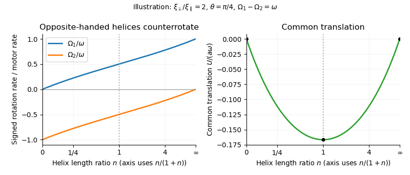
Counterrotation rates and common translation versus the right-to-left helix length ratio, showing no propulsion at zero or infinite ratio and symmetric counterrotation for equal lengths
. Details. Past exam of the mathematics course of the University of Cambridge 2016 iii Paper 334 3 Solution Created 2026-10-03 Updated 2026-10-06
In resistive-force theory (RFT), the hydrodynamic force per unit arclength exerted by the fluid on a slender filament isHere is the unit tangent and the local velocity relative to the background fluid. The parallel and perpendicular drag coefficients of a slender filament are positive and generally satisfy ; their leading logarithmic ratio is about two. This local approximation assumes a small filament radius compared with length and curvature scales, negligible fluid inertia, and a Newtonian fluid. It represents drag by the local tangent direction and neglects nonlocal hydrodynamic interactions between separated filament segments. Boundaries, close approaches and end corrections may require slender-body theory or a more complete flow calculation. In this problem the background fluid is at rest, and the drag coefficients are taken uniform along the filament.
The rigid-body velocity in a deforming swimmer frame is the sum of translation, rotation and material deformation. With ,so, in instantaneous swimmer-frame components,The reference-frame conditions attach the origin and orientation to the filament's base and base tangent. They prevent arbitrary shape translations or tilts from being absorbed into the definition of .
The exact tangent and arclength element areSince , the local velocity is . Changing the drag tensor by its tangent correction therefore changes only at . The arclength correction is smaller still at this order. Also . Thus is sufficient at order . This assumes the small-slope expansion is uniform, .
Put and , with . The first-order local force isIts total hydrodynamic forces areTaking the moment about the swimmer-frame origin, , the second term is beyond first order. HenceFor force-free and torque-free motion, the three leading coefficients vanish. The longitudinal force immediately gives . The two transverse equations areTheir determinant is . Solving yields the first-order free swimming of a planar filament:The resistive-force theory coefficient cancels because both equations use the same transverse drag. Another interpretation is the least-squares projection of filament deformation velocity: is the best affine approximation to on . Zero transverse force and torque mean that the residual is orthogonal to and .
If is sufficiently differentiable and periodic with period , each has zero temporal mean. More explicitly,Both bracketed quantities return to their initial values over a period. Thus the first-order periodic transverse swimming velocity satisfiesThese results concern first order and swimmer-frame components. Changes of orientation can affect laboratory displacements at second order; higher-order net swimming is not ruled out.
Past exam of the mathematics course of the University of Cambridge 2016 iii Paper 334 2 Solution Created 2026-10-03 Updated 2026-10-14
Use and in the frame translating with the sheet. At each instant, the incompressible Stokes equations areTaking their curl gives the biharmonic stream function for planar Stokes flow:in the fluid above the actual sheet. The no-slip boundary condition is imposed on material points, whose label is and whose actual horizontal position is . With ,The second sign follows from . Far above the sheet,with bounded velocity and no imposed mean pressure gradient. The positive far-field velocity arises because the sheet moves with laboratory velocity . All fields are -periodic in ; an additive function of time in is a harmless gauge. These conditions formulate the Taylor swimming sheet problem with both types of travelling deformation.
Expand and . At first order the boundary can be evaluated at :The far-field conditions are and . For a nonzero Fourier mode of wavenumber , bounded velocity selects ; the exponentially growing modes are excluded. Matching the modes and givesAn additive gauge has been set to zero. The first term is a transverse mode of a Taylor swimming sheet, and the second is a longitudinal mode of a Taylor swimming sheet. Their velocities decay at infinity. The mean first-order boundary velocity is zero, and the bounded zero Fourier mode is a constant plus a multiple of , so .
For the second-order Taylor-expanded no-slip boundary condition, the first-order displacement isThere is no explicit second-order material velocity in the prescribed motion. Hence, with all first-order derivatives evaluated at ,where and . Differentiation of the first-order solution giveson the flat reference boundary. ThereforeThe boundary conditions for the streamfunction are and . Their far-field counterparts are and .
Products of the two distinct first-order Fourier modes generate only the nonzero wavenumbers , as well as a mean. Thus the bounded general solution compatible with these data has the formThe discarded zero-mode terms would give unbounded velocity, and the discarded nonzero modes grow exponentially. The zero-mean normal velocity in periodic half-space Stokes flow is consistent with a bounded periodic flow and no far-field vertical flux. For example, integrating along the boundary yieldsThis fixes the ; the nonconstant part of fixes . All coefficients are thereby determined, but none is needed to find the mean swimming speed.
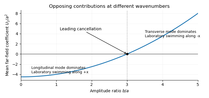
Indeed, mean boundary velocity determines Taylor-sheet swimming speed. The mean Fourier mode of is , so its horizontal velocity is the same at the boundary and infinity. Fourier orthogonality of sheet swimming modes removes the mixed product, givingHere is the average over one spatial period; a temporal average gives the same answer for these travelling waves. The laboratory swimming velocity is . The transverse wave drives motion opposite to its direction of propagation, whereas the longitudinal wave drives it in the propagation direction. Their wavenumbers enter quadratically. Thus cancels the swimming speed at order . This different-wavenumber cancellation in sheet swimming is not a claim that all higher-order swimming terms vanish.
Past exam of the mathematics course of the University of Cambridge 2016 iii Paper 334 1 Solution Created 2026-10-03 Updated 2026-10-14
Let be the dynamic viscosity, , and the signed force exerted by sphere on the fluid. For negligible sphere inertia, this also equals the externally or internally applied force on that sphere; its hydrodynamic force is . The Stokes drag law and the axial velocity of a Stokeslet give the leading hydrodynamic mobility matrixThe factor follows from when is parallel to the line of centres. The longitudinal two-sphere mobility retains the first interaction in ; finite-size and repeated-reflection corrections are higher order.
For the linked force-free pair, . Put and . ThensoThe coefficient depends only on the current separation. For any period , , and thereforeThis is a closed integral of a single-valued function of one real shape coordinate. Since and , both spheres also have zero net displacement. Equal radii make instantaneously; unequal radii generally permit oscillatory translation, but still no mean motion. This explicit force-free two-sphere stroke is the scallop theorem: a single-parameter reciprocal deformation in a Newtonian fluid at zero inertia cannot produce net free swimming. The timing of extension and contraction cannot change that conclusion, because Stokes flow has no inertial memory.
For the externally prescribed pair, put , , andInvert the hydrodynamic mobility matrix:In a large- expansion with fixed,The isolated-drag term and the constant- interaction have zero mean. The order- term from also has zero mean, since its coefficient is constant at that order. Meanwhile,Consequently the externally driven two-sphere pump has the following phase-dependent mean force of an externally driven sphere pair:Here denotes averaging over one period. The analogous calculation gives , so at leading order, andThus the mean fluid forcing is nonzero except at or modulo . The sign changes when the phase lag is reversed. Those exceptional strokes are reciprocal: the position-space loop collapses to a line, and their mean force vanishes by reversibility, not just by this leading expansion.

An externally driven two-sphere stroke with phase lag pi over three encloses a position-space loop, and its leading mean fluid force varies as the sine of the phase lag
. Details. There is no contradiction with the scallop theorem. The externally imposed motion is not force-free, and the actuators prescribe two phase-shifted motions; their combined motion is not reciprocal for a generic phase. The spheres return to their prescribed positions while transferring a mean force to the fluid. This is pumping by external forcing, rather than propulsion of the freely linked one-shape-coordinate system.
The asymptotic calculation requires and persistent large separation. The minimum separation of phase-shifted sphere oscillations isThe printed condition alone does not guarantee nonoverlap or the stipulated far-separated regime. The prescribed trajectories must additionally keep this minimum well above both radii. This is a compatibility qualification on the data, not a change of the phase-dependent force calculation.
Past exam of the mathematics course of the University of Cambridge 2016 iii Paper 333 2 Solution Created 2026-10-03 Updated 2026-10-06
The vertical component is times the first-order anomaly in shallow-water potential vorticity about rest:Thus records the combination of relative vorticity and column stretching that is conserved by the unforced linearized shallow water equations. Indeed their curl and continuity equation give . It is the persistent forcing of the balanced component during geostrophic adjustment, while inertia-gravity waves carry away the unbalanced component.
Initially . In the final geostrophic flow, , , and . Conservation of the linearized shallow-water potential vorticity therefore givesBoundedness on both sides and continuity of at the origin determine the constants:The solution is the locally attained balanced state after outgoing inertia-gravity waves have departed; the full inviscid system need not lose its globally conserved wave energy. The signed volume flux in the direction is
For double Kelvin-wave adjustment at a depth step, put and use on the corresponding side of the step. The PDF's far-field wording must mean , rather than for every . In the exponentially trapped outer response, cross-step geostrophic balance gives, at ,To retain the propagation of this slowly varying trapped disturbance, the along-step acceleration in must also be retained. It supplies the small cross-step ageostrophic flow. Thus the two cross-step volume fluxes areHere as a distributional derivative. Equating the fluxes and dividing by givesThe printed forcing is missing a factor of two. It cannot follow from the printed sign-function surface profile with the usual Dirac delta distribution normalization. Pure geostrophic balance in both horizontal directions would also omit and could not determine the wave evolution.
The method of characteristics with zero initial amplitude gives the corrected weak solutionBehind the eastward front, , the surface elevation at the step becomes , matching the upstream side. All the original cross-step transport is diverted into flow along the step once the wave has passed a fixed location: there, with opposing along-step velocities above and below the step. This is the complete barrier in the adjusted region, and in the long-time limit at every fixed . At finite time a front still carries cross-step flux: the formulas above give . The discontinuous outer representation does not resolve the short-scale fast adjustment at either front.
For completeness, solving the equation literally as printed instead gives . Its amplitude is half that required; retains a jump at the origin after passage, so that literal equation does not imply complete blocking. The corrected equation and the literal printed equation are distinguished rather than asserting an inconsistent barrier result.
Past exam of the mathematics course of the University of Cambridge 2016 iii Paper 333 1 Solution Created 2026-10-03 Updated 2026-10-06
Use an upward vertical coordinate , constant mass density , and a positive Coriolis parameter ; the square-root formulas below assume the Northern Hemisphere. For a slab of thickness , the net force per unit horizontal area is . Dividing by its mass and including the Coriolis acceleration givesHere are the vertical shear stress components of the viscous stress tensor, so their boundary values require a signed traction convention. Linearization removes advective acceleration. Decompose the horizontal velocity into an exterior pressure response and an Ekman layer correction. On an f-plane these satisfyandThe exterior pressure response is in geostrophic balance when steady. For a surface Ekman layer with negligible stress at its base, its Ekman transport isIntegrating the continuity equation and imposing zero vertical boundary-layer velocity at the surface gives . Thus the base velocity, positive upward, isThe PDF prints the opposite sign. Its negative formula is correct for a velocity defined positive downward, but its stated momentum equations with use the upward-coordinate shear convention above. This sign must be accounted for when interpreting the subsequent pumping equation.
For constant kinematic viscosity, write and . The steady Ekman layer equation is . Taking the surface at and the ocean below it, the bounded surface Ekman layer solution isThe total velocity is . Prescribed wind stress determines the coefficient of this Ekman layer correction; it does not determine a relation between the wind and the independent pressure-driven velocity. An additional boundary condition is necessary for a laminar Ekman boundary stress law in terms of .
The two printed laminar stress formulas and the positive pressure-Laplacian pumping formula are instead the standard Bottom Ekman layer relations. To derive them consistently, put a stationary no-slip boundary condition at , with water at . ThenConsequentlyThese are shear stress values; the actual bottom traction on the fluid has the opposite sign. Integrating this Bottom Ekman layer gives and . Since the exterior geostrophic flow is horizontally nondivergent, the upward velocity above the bottom is . Using , yieldsThis recovers the requested magnitude and pressure dependence with a consistent bottom interpretation. The surface version would require its own specified boundary velocity and corresponding signs.
For Ekman spin-down in a shallow-water layer, let , , and . Upward bottom pumping enters the exterior linearized shallow water equations through . Taking the curl of their momentum equations gives , henceSlow geostrophic balance gives and . Therefore the intended damping equation isThe slow-adjustment assumption is , not the printed . The printed negative pumping term in continuity can alternatively describe downward extraction at the upper boundary, but it cannot be combined unchanged with the upward bottom pumping just derived. A literal use of the positive printed and negative continuity source would reverse the damping sign and produce growth.
For a Fourier mode with , substitution givesFor scales small compared with the Rossby deformation radius, and , independent of wavenumber. For scales large compared with the Rossby deformation radius, the equation becomes , whereThe zero wavenumber mode does not decay. A thin Ekman layer, , makes , so the derived decay time satisfies the corrected slow-time assumption.
Past exam of the mathematics course of the University of Cambridge 2016 iii Paper 332 3 Solution Created 2026-10-03 Updated 2026-10-14
Take upward from the horizontal bed and measure away from an ice divide. In the shallow-ice approximation, the hydrostatic pressure is and the horizontal balance for a Newtonian fluid isThe upper stress-free boundary condition gives . The resisting basal traction is , so the fluid-side shear stress satisfies . This is a Navier slip boundary condition with slip length . Integrating twice givesThe first term is the uniform basal sliding contribution, while the quadratic term is internal viscous deformation. Both are positive where the thickness decreases downstream.
The shallow-ice flux with linear basal drag isNo ice accumulation or ice ablation appears. For a symmetric glacier, work on one half, , with , and no outgoing volume flux. Its conserved half-volume per unit width is ; the full glacier has volume . This specifies the volume convention rather than silently supplying an unspecified value. For a general finite release on the whole line, the late similarity solution is centred on its conserved centre of mass and uses half its total volume for .
The internal-shear and linear basal drag law mobilities are equal at . Suitable vertical, horizontal and temporal scales areWrite , , . ThenThe initial typical thickness is , the initial extent is of order , and its shear-controlled spreading time is of order . The shallow-ice approximation also requires small aspect ratio: in particular the initial thickness and extent must satisfy approximately . The equations model the broad shallow bulk; the very tip can require physics beyond that approximation.
The two limiting equations are porous medium equations of the form , with for a thick shear-dominated glacier and for a thin sliding-dominated glacier. Volume conservation and balance of the time derivative give exponent . Set , . One integration, using zero volume flux at the ice divide, gives , henceThe planar volume-conserving nonlinear-diffusion similarity is thereforeThe Beta function fixes its constants:Consequently the explicit early shear and late sliding limits areTheir centre depths are with , and with . Thus the early extent grows as and the late extent as . These are asymptotic regime profiles; they solve the respective limiting equations, not the full sum of both mobilities. For arbitrary finite-width initial data they are appropriate after the corresponding spatial relaxation, with a virtual time origin depending on that data.
The shear-to-slip transition in a shallow ice current occurs at thickness of order . Using equality at the centre of the early similarity solution givesIf the initial profile is already approximated by that early similarity solution and its centre depth is 10, the virtual age is , and the elapsed estimate is . Other reasonable definitions of typical thickness change the order-one coefficient; the initial thickness alone does not uniquely determine an exact transition time or an exact initial profile. The robust nondimensional estimate is a transition time of order one in the scale.
Finally, let a local nose translate steadily at positive speed and write . This is a local traveling nose of a glacier with linear basal drag; the speed of the globally spreading glacier changes slowly with time. The local mass conservation equation integrates to , since both and vanish at the front. Therefore
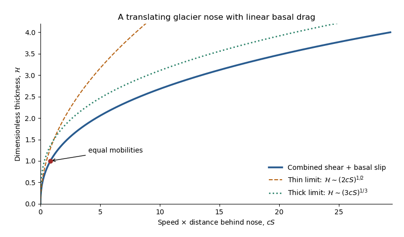
The right side is strictly increasing, giving a unique positive thickness at every . With and , the same relation reads . Its limiting profiles areThe square-root tip reflects basal sliding; the cube-root thicker region reflects internal viscous deformation. Even during the early thick regime, the very nose is thin and has the square-root inner form. At late times that sliding balance governs nearly the whole profile. The dimensionless crossover thickness is and its distance is ; the early thick cube-root outer profile matches this smaller sliding region. The diverging geometric slope at the idealized tip also marks the local limit of the long-wave shallow-ice approximation.
Past exam of the mathematics course of the University of Cambridge 2016 iii Paper 332 2 Solution Created 2026-10-03 Updated 2026-10-06
Choose the positive direction along the background flow, so ; reverse if necessary. Let measure depth below the impermeable roof, and set . The deep ambient water has . Continuity of pressure at and hydrostatic pressure inside the buoyant CO2 giveHere is permeability of a porous medium and is dynamic viscosity. Since , the ambient return-flow correction to the imposed pressure gradient is higher order. The small aspect ratio supplies the hydrostatic pressure approximation; capillary trapping, dissolution, compressibility and dispersion are omitted in this sharp-interface model.
The depth-integrated Darcy flux is . The actual stored fluid volume is per unit horizontal area, where is the aquifer porosity. Thus the porous gravity current with background flow satisfieswith , and . Both and the later denote actual injected volume per unit transverse width. Away from injection, the equation is an advected porous medium equation. At each finite front impose and vanishing outgoing volume flux per unit width. At the injection point is continuous and . For an initially empty aquifer, . The advective speed is , not .
For a constant-flux porous gravity current, write characteristic depth and extent temporarily. At early times volume conservation gives ; gravity spreading gives . HenceBackground advection becomes comparable when , so the transition scales areFor , the leading similarity solution is symmetric:For , its model ordinary differential equation and boundary conditions areChoose the nonnegative finite-front branch, reflect evenly in , and require at the front. The factor divides the injection equally between the two halves. Integration of the ordinary differential equation gives ; the limiting front slope is . This boundary-value problem determines the initially symmetric shape without assuming an unjustified elementary formula. Independent numerical integration gives in this normalization.
For , upstream storage approaches a finite steady value. With no upstream leakage, for , giving wherever . Downstream the uniform interior carries , soThe upstream volume flux vanishes even though local Darcy velocity contributions from background flow and buoyancy cancel. The upstream stored volume is , a finite constant. The downstream plateau therefore extends a distance , and its front advances at to leading order.
The diffusive nose of an advected porous gravity current has widthIn a frame translating at , balance the time derivative against the nonlinear gravity diffusion. With and , the leading transition is , withIts finite front has as . Independent numerical integration of this boundary-value problem gives , so a more accurate leading nose position is and its local shape is . The entire transition has no elementary closed form. A useful explicit, approximate shape is the volume-preserving linear rampThis gives . Its ramp width is , and its edge obeys the exact kinematic boundary condition to the displayed order. It also has the same area as a sharp step at . This is an approximate ramp closure, not an exact solution of the nonlinear nose ordinary differential equation. A constant phase shift balances the finite upstream storage within this ramp approximation; the full solution's subleading matching may alter constant offsets.
For a rapid injection of total volume , remove the source for and introduce . The advected constant-volume porous gravity current obeys and . A similarity solution has depth proportional to and radius proportional to . Direct substitution gives the compactly supported Barenblatt solutionIndeed . Its centre translates at the pore speed , its two edges are , and its maximum depth decays as . The expression is exact for a point release within this reduced model; finite-width initial data approach this similarity solution at late times. If , the constant-rate current remains in the symmetric spreading regime and the constant-volume solution has a stationary centre.
Past exam of the mathematics course of the University of Cambridge 2016 iii Paper 332 1 Solution Created 2026-10-03 Updated 2026-10-14
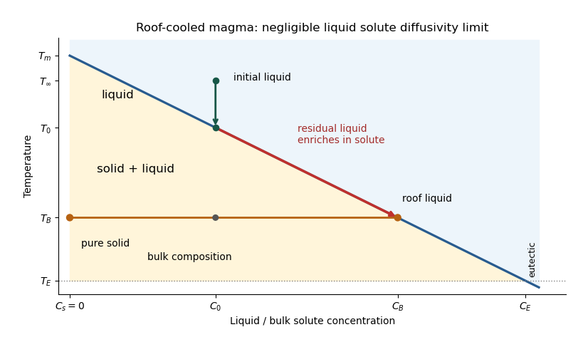
Take positive downwards from the roof. Write , , and . The cooled magma follows the decreasing liquidus from towards ; the initially superheated liquid starts at above that liquidus. The solid has zero solute concentration. At each temperature in the mushy layer, a horizontal tie line joins the pure solid to the residual liquid on the liquidus. The lever rule gives the liquid fraction from the bulk concentration. Since , this path stops before the eutectic temperature and does not cross the eutectic composition.


The porosity denotes the liquid fraction, so is the solid fraction. Equal phase mass densities remove volume-change flow; the stable density stratification suppresses convection. In the stagnant mushy-layer model, define bulk specific enthalpy and bulk solute concentration byThe arbitrary reference of specific enthalpy has been omitted. The two conservation laws in areHere is the thermal diffusivity, with the thermal conductivity. The positive term records increased specific enthalpy on melting; during freezing it supplies latent heat. In the liquid , the heat equation and solute diffusion equation arewhere is the solutal diffusivity. Neglecting solute diffusion inside the mushy layer does not permit dropping in the liquid at this stage.
Use , liquid and as , and initially , , for . These are the half-space boundary conditions appropriate before cooling reaches the bottom of the chamber. For a closed chamber of finite depth , replace the far-field conditions by the specified bottom conditions, for example at an insulated impermeable floor; the half-space similarity solution then ceases to apply when the thermal penetration depth approaches .
At , let and be the common liquid concentration and temperature, and let be the limiting porosity on the mush side. Continuity of , the Rankine-Hugoniot condition for solute, and the interfacial conservation of energy giveThe first condition has the sign of solute rejection into the liquid. For the sharp-edge stagnant mushy-layer model with nonzero liquid solutal diffusivity, close the free-boundary problem by marginal equilibrium at a mush-liquid boundary:This prevents constitutional supercooling immediately ahead of the mushy layer. A small solid fraction jump at its edge is allowed: imposing as well as these finite- conditions would generally overdetermine the reduced model. At the roof, follows from the liquidus, and no additional solute-flux boundary condition is needed in the diffusion-free mush.
To obtain the large-concentration similarity solution, putThe positive superheat specifies the physically intended liquid initial state. On a similarity solution, are constant, so every newly incorporated level leaves the same constant . Write and . Then throughout the mushy layerFor , , and , the effective heat capacity is constant to relative error . Thus setIntegration of the similarity solution ordinary differential equation gives the leading analytical profilesThe temperature is . In the mushy layer, the concentration and porosity are the displayed ; in the liquid,These retain the liquid solutal boundary layer. For completeness, finite- values of are determined analytically, to the same large- order, by settingand solvingThe solute jump gives exactly; replacing by on the right of the last equation retains that jump's next-order factor, but does not make the linearized thermal profiles exact at finite . The branch has , . All these profiles are leading asymptotic expressions, not exact solutions of the nonlinear finite- heat equation.
For at fixed positive , the complementary error function asymptotic gives , hence , , , and . The result simplifies toIn particular, and . There is no finite interfacial latent heat jump in this limit: the latent heat is released continuously throughout the mushy layer. Matching the two temperature gradients givesThe printed final equation is missing the square on in the exponential. The corrected exponent follows directly from differentiating and is consistent with . The positive root is unique: the mush-side gradient decreases from infinity to zero with , whereas increases. The zero-superheat limit is singular and is not described by a finite positive in this two-region construction.
There are unlisted articles, also show them or only show them.