
Past exam of the mathematics course of the University of Cambridge 2020 ii Paper 2 9D ii Solution Created 2026-09-24 Updated 2026-09-29
For and , putThe slow-roll approximation gives andTherefore, with ,Since , integration of the Hubble parameter gives
Past exam of the mathematics course of the University of Cambridge 2020 ii Paper 2 9D i Solution Created 2026-09-24 Updated 2026-09-29
Past exam of the mathematics course of the University of Cambridge 2020 ii Paper 2 6B iii Solution Created 2026-09-24 Updated 2026-09-29
Along a solution, the chain rule and antisymmetry of givebecause for every real vector . ThereforeThe closed level curves around the strict minimum at the coexistence equilibrium are the periodic population cycles of the Lotka-Volterra predator-prey model.
Past exam of the mathematics course of the University of Cambridge 2020 ii Paper 2 6B ii Solution Created 2026-09-24 Updated 2026-09-29
Since , division of each population equation by givesDefine the Hamiltonian functionand the antisymmetric matrixThen
Past exam of the mathematics course of the University of Cambridge 2020 ii Paper 2 6B i Solution Created 2026-09-24 Updated 2026-09-29
At a nonzero fixed point, both bracketed per-capita growth rates vanish:Hence the coexistence equilibrium of this Lotka-Volterra predator-prey model is
Past exam of the mathematics course of the University of Cambridge 2020 ii Paper 2 5J c Solution Created 2026-09-24 Updated 2026-09-29
Let be independent standard logistic random variables and define the latent variableSet exactly when . If is the logistic cumulative distribution function, its symmetry and the identity givewhich is precisely the fitted logistic regression.
Past exam of the mathematics course of the University of Cambridge 2020 ii Paper 2 5J b Solution Created 2026-09-24 Updated 2026-09-29
Two packs contain cigarettes. Holding height fixed, increasing average consumption from zero to two packs per day changes the log odds byThe corresponding odds ratio is thereforeThus the model estimates that a two-pack-per-day smoker has about times the odds of heart disease of an otherwise comparable nonsmoker. This is an association in the fitted observational model, rather than by itself a causal conclusion.
Past exam of the mathematics course of the University of Cambridge 2020 ii Paper 2 5J a Solution Created 2026-09-24 Updated 2026-10-03
Let be the indicator that man develops heart disease and let . The fitted logistic regression assumes independent Bernoulli responses with
Past exam of the mathematics course of the University of Cambridge 2020 ii Paper 2 4F ii Solution Created 2026-09-24 Updated 2026-09-29
The setis the diagonal halting set. It is recursively enumerable by simulating the coded machine, but it is not recursive by the halting problem diagonal argument.
By contrast, is recursive: decode , reject it if it is not a program code, otherwise simulate the program on input for exactly steps and accept precisely if it has halted. This bounded computation always terminates. Thus
Past exam of the mathematics course of the University of Cambridge 2020 ii Paper 2 4F i Solution Created 2026-09-24 Updated 2026-09-29
A subset is recursive when its indicator function is a total computable function. It is recursively enumerable when it is the domain of a partial computable function, equivalently when an algorithm can enumerate its members.
If is recursive, its indicator decides both and its complement, so both sets are recursively enumerable. Conversely, suppose programs enumerate and . On input , run the two enumerations in parallel by dovetailing. Exactly one must eventually print ; accept in the first case and reject in the second. This algorithm always halts and decides . Hence
Past exam of the mathematics course of the University of Cambridge 2020 ii Paper 2 40E d Solution Created 2026-09-24 Updated 2026-09-29
Because is a positive-definite matrix, it has a positive-definite inverse square root. Choose the exact inverse-square-root preconditionerThenwhich has one distinct eigenvalue, so preconditioned CG terminates in one step.
This construction is of little computational use because obtaining and applying is generally at least as expensive in storage and arithmetic as directly factoring or solving the original system. A useful preconditioner must only approximate this transformation while remaining cheap to construct and apply.
Past exam of the mathematics course of the University of Cambridge 2020 ii Paper 2 40E c Solution Created 2026-09-24 Updated 2026-09-29
Let . The displayed lower-bidiagonal matrix satisfiesSince , the Preconditioned conjugate gradient method usesSolving givesThe rank-one matrix has eigenvalue in the direction and eigenvalue on the -dimensional orthogonal complement of . It therefore has only two distinct eigenvalues. Part (b) gives
Past exam of the mathematics course of the University of Cambridge 2020 ii Paper 2 40E b Solution Created 2026-09-24 Updated 2026-09-29
For an iterate , the Conjugate gradient method residual isTwo fundamental properties are the Conjugate-gradient residual orthogonality conditionsEquivalently, the residuals generated before convergence are mutually orthogonal and span the successive Krylov spaces.
Since has only distinct eigenvalues, its minimal polynomial has degree at most . ConsequentlyThe two properties then put both inside and orthogonal to , so . Hence , and
Past exam of the mathematics course of the University of Cambridge 2020 ii Paper 2 40E a Solution Created 2026-09-24 Updated 2026-09-29
The th Krylov subspace isBecause has a complete eigenbasis, decomposewhere is the projection of onto the eigenspace belonging to the th distinct eigenvalue ; some may vanish. ThenEvery generator of therefore belongs to , and
Past exam of the mathematics course of the University of Cambridge 2020 ii Paper 2 3I b ii Created 2026-09-24 Updated 2026-09-24
Past exam of the mathematics course of the University of Cambridge 2020 ii Paper 2 3I b i Created 2026-09-24 Updated 2026-09-24
Past exam of the mathematics course of the University of Cambridge 2020 ii Paper 2 3I a Solution Created 2026-09-24 Updated 2026-09-29
For a discrete memoryless channel with input and output , its information capacity iswhere is the mutual information and the maximum is over all input distributions. Capacity is measured in bits when logarithms have base two.
Past exam of the mathematics course of the University of Cambridge 2020 ii Paper 2 39B c Solution Created 2026-09-24 Updated 2026-10-14
Take a linear combination of the P- and SV-fields from part (b). The rigid boundary condition at givesThe conditions at are the same because the horizontal displacement is even and the vertical displacement is odd. A nonzero pair exists exactly when the determinant vanishes:Therefore the rigid elastic waveguide mode dispersion relation is
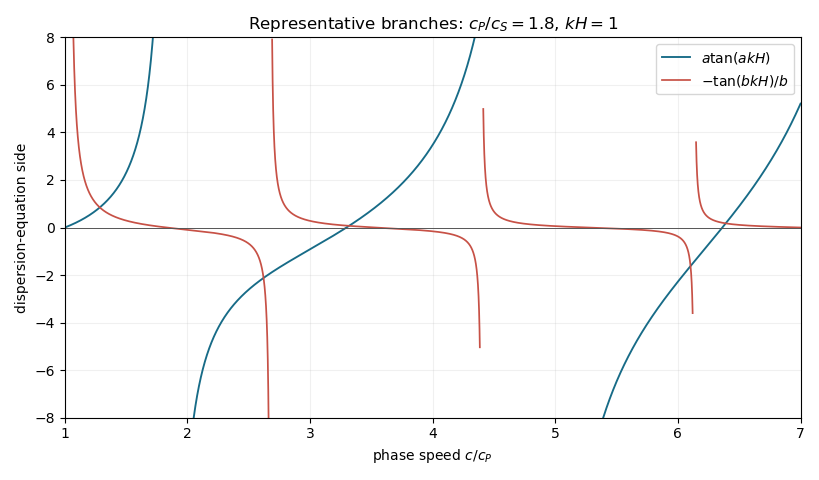
Dispersion relation branches in an elastic waveguide
. Details. 
As increases, both and increase without bound. The two sides consequently have infinitely many alternating tangent branches and poles. On successive continuity intervals their relative ordering reverses, so the intermediate value theorem gives infinitely many intersections, corresponding to infinitely many propagating waveguide modes.
Past exam of the mathematics course of the University of Cambridge 2020 ii Paper 2 39B b Solution Created 2026-09-24 Updated 2026-09-29
Past exam of the mathematics course of the University of Cambridge 2020 ii Paper 2 39B a Solution Created 2026-09-24 Updated 2026-10-14
Substitute the harmonic plane waveinto the elastic wave equation. The vector identitygivesIf is parallel to , this becomesand gives a longitudinal P wave. If , it becomesand gives either polarization of an S wave.
For , convenient polarization vectors areThe SV-wave lies in the propagation plane, whereas the SH-wave is perpendicular to that plane.
There are unlisted articles, also show them or only show them.