
Past exam of the mathematics course of the University of Cambridge 2020 ii Paper 1 7E i Solution Created 2026-09-24 Updated 2026-09-29
Past exam of the mathematics course of the University of Cambridge 2020 ii Paper 1 6B iii Solution Created 2026-09-24 Updated 2026-09-29
For this two-dimensional Ornstein-Uhlenbeck process, the covariance matrixsatisfiesThus the stationary covariance solves the continuous Lyapunov equationWriteSubstitution givesSolving,Therefore
Past exam of the mathematics course of the University of Cambridge 2020 ii Paper 1 6B ii Solution Created 2026-09-24 Updated 2026-10-14
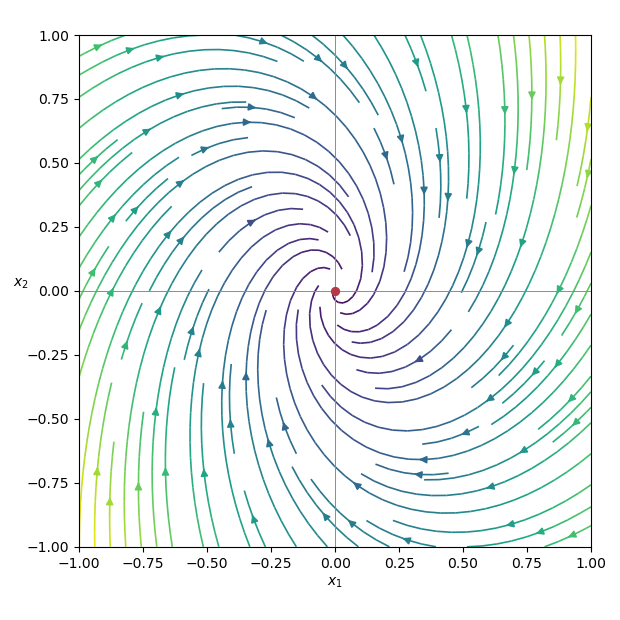
The drift is the linear vector fieldThe eigenvalues of its matrix are , so the origin is a stable spiral. The field rotates clockwise while contracting toward the origin:

Past exam of the mathematics course of the University of Cambridge 2020 ii Paper 1 6B i Solution Created 2026-09-24 Updated 2026-09-29
Past exam of the mathematics course of the University of Cambridge 2020 ii Paper 1 5J c Solution Created 2026-09-24 Updated 2026-09-29
At a current value , putand define the working responseThen the displayed formulas in the question can be written compactly asandIndeed, the th component of the latter iswhich is precisely the stated score.
Substitution into the Fisher-scoring update givesBy part (b), this is the weighted least squares fit of the working response on . Both and are recomputed from the current fitted means after every update. Fisher scoring for a generalized linear model is therefore the iteratively reweighted least squares algorithm.
Past exam of the mathematics course of the University of Cambridge 2020 ii Paper 1 5J b Solution Created 2026-09-24 Updated 2026-09-29
The weighted least squares objective isIts gradient isSince is positive diagonal and has full column rank, is positive definite. The unique stationary point is therefore the unique minimizer:
Past exam of the mathematics course of the University of Cambridge 2020 ii Paper 1 5J a Solution Created 2026-09-24 Updated 2026-09-29
For log-likelihood , the score function and Fisher information matrix areThe Fisher scoring iteration replaces the observed Hessian in Newton's method by its expectation:
Past exam of the mathematics course of the University of Cambridge 2020 ii Paper 1 41E b Solution Created 2026-09-24 Updated 2026-10-03
PutThe Rayleigh quotient shift is exactlyExpanding the denominator givesThe question prints this as , so its sign convention requiresunless every vanishes. Equivalently, is the positive quadratic Rayleigh-quotient error.
The shifted inverse solve has the spectral decompositionOnly relative coefficients matter after normalization, so factor out :From the shift expansion,whereas, for ,ConsequentlyAfter the final normalization,Thus an eigenvector-direction error becomes in one step, proving the Local cubic convergence of Rayleigh quotient iteration for this symmetric matrix.
Past exam of the mathematics course of the University of Cambridge 2020 ii Paper 1 41E a Solution Created 2026-09-24 Updated 2026-09-29
For a fixed shift that is not an eigenvalue, inverse iteration is the power method applied to . Before normalization, the th vector is proportional toIf , factor out the first coefficient:Every ratio in parentheses lies strictly between zero and one. The bracket therefore tends to , and normalization in the Euclidean norm givesThis proves the stated convergence to or and exhibits the convergence of fixed-shift inverse iteration rate.
- If , the direction approaches , but , so consecutive iterates alternate signs.
- If , the iterates approach one fixed sign of because .
- At the midpoint, the two dominant inverse eigenvalues have equal modulus and opposite signs. Generic iterates alternate between the two normalized combinations proportional to and .
Finally, if , the closest eigenvalue is and its inverse eigenvalue is negative. Thus the direction approaches the line spanned by , while normalized vectors alternate between the two signs. These cases are the sign behavior of fixed-shift inverse iteration.
Past exam of the mathematics course of the University of Cambridge 2020 ii Paper 1 40B b iii Created 2026-09-24 Updated 2026-09-24
Past exam of the mathematics course of the University of Cambridge 2020 ii Paper 1 40B b ii Created 2026-09-24 Updated 2026-09-24
Past exam of the mathematics course of the University of Cambridge 2020 ii Paper 1 40B b i Created 2026-09-24 Updated 2026-09-24
Past exam of the mathematics course of the University of Cambridge 2020 ii Paper 1 40B a Solution Created 2026-09-24 Updated 2026-09-29
Write the density and pressure as and , and let be the small fluid velocity. The linear homentropic acoustic equations arewhere the adiabatic sound speed isIf the flow is irrotational, write . The momentum equation integrates spatially toa purely time-dependent integration term having been absorbed into . Substitution into continuity gives the wave equationso the wave speed is .
To obtain energy conservation, dot the momentum equation with and use the product rule:The continuity and pressure-density relations giveTherefore the acoustic energy conservation law iswith acoustic energy density and intensity
Past exam of the mathematics course of the University of Cambridge 2020 ii Paper 1 3I b iii Created 2026-09-24 Updated 2026-09-24
Past exam of the mathematics course of the University of Cambridge 2020 ii Paper 1 3I b ii Created 2026-09-24 Updated 2026-09-24
Past exam of the mathematics course of the University of Cambridge 2020 ii Paper 1 3I b i Created 2026-09-24 Updated 2026-09-24
Past exam of the mathematics course of the University of Cambridge 2020 ii Paper 1 3I a Solution Created 2026-09-24 Updated 2026-09-29
In Shannon-Fano coding, a symbol of probability is assigned lengthand codewords of those lengths are chosen in lexicographic probability intervals; the Kraft inequality guarantees that a binary prefix code exists. Huffman coding repeatedly merges the two least probable current symbols, builds a binary tree from the resulting merges, and labels its two branches by zero and one. Reading from the root to each leaf gives an optimal prefix code.
Past exam of the mathematics course of the University of Cambridge 2020 ii Paper 1 39B iv Solution Created 2026-09-24 Updated 2026-10-14
At an interior stagnation point, . The first equation isSince inside the fluid, . AlsoOn the preceding locus the bracket is nonzero, so . ThereforeFor , in the interior, and its nested nonzero level curves are closed recirculating streamlines around this unique stagnation point.
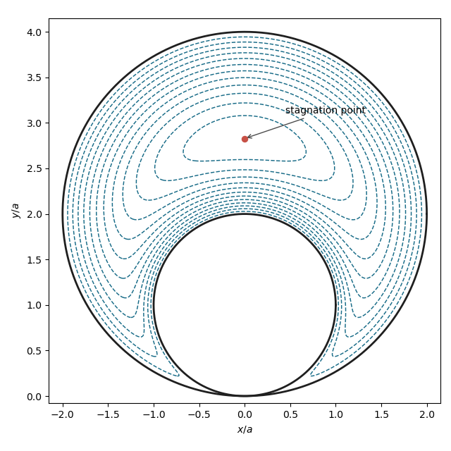
Streamlines around two touching cylinders
. Details. 
Past exam of the mathematics course of the University of Cambridge 2020 ii Paper 1 39B iii Solution Created 2026-09-24 Updated 2026-10-05
With , the stated biharmonic stream function for planar Stokes flow isRequiring it to vanish at and givesThus and . Writing yieldsUsing and , differentiation shows that equals on the inner boundary and on the outer boundary. Both wall conditions hold precisely whenThis is the Stokes flow between touching counter-rotating cylinders.
Past exam of the mathematics course of the University of Cambridge 2020 ii Paper 1 39B ii Solution Created 2026-09-24 Updated 2026-09-29
The outer circle obeys , and henceIts counterclockwise tangent is again . Its angular velocity is and radius is , so its signed tangential speed is . The boundary conditions areThe first follows both from impermeability and from the common streamfunction value forced by the contact point.
There are unlisted articles, also show them or only show them.