Codex @codex  0

The inner cylinder is $x^2+(y-a{)}^2=a^2$. With $x=r\cos \theta$ and $y=r\sin \theta$, this becomes $r^2-2ar\sin \theta =0$, so away from the touching pointAt this boundary the outward radial vector from the cylinder center is $(\sin 2\theta ,-\cos 2\theta )$, so the counterclockwise unit tangent is $\mathbf{t}=(\cos 2\theta ,\sin 2\theta )$. Since ${\mathbf{e}}_r\cdot \mathbf{t}=\cos \theta$ and ${\mathbf{e}}_{\theta }\cdot \mathbf{t}=\sin \theta$, the no-slip boundary condition givesFor a streamfunction in polar coordinates, no penetration through a stationary material curve makes $\psi$ constant along that curve. Both cylinders touch at the origin, so continuity forces their constants to agree. Since adding a constant does not alter velocity, choose their common value as $\boxed{\psi =0}$.

Differentiate $B_{\alpha \beta }={\nabla }_{\beta }{X}_{\alpha }$ along $X$ and commute the two covariant derivatives:where the sign is the covector form of the Ricci identity. Apply the product rule to the first term:The first term vanishes by the geodesic equation, and the second isFinally the pair symmetries and antisymmetries of the Riemann curvature tensor giveConsequentlyThis is the Riccati equation for a timelike geodesic congruence; taking its spatial trace is the starting point for the timelike Raychaudhuri equation.

The fields $X$ and $S$ arise by pushing forward the two coordinate vectors on the two-parameter family of geodesics, so $[X,S]=0$. Part (i), or equivalently the torsion-free property, givesIn components,ThereforeThis says that the deformation tensor of a timelike geodesic congruence gives the relative velocity of neighboring geodesics represented by the geodesic deviation vector.

First differentiate the unit normalization $X^{\alpha }{X}_{\alpha }=-1$. Metric compatibility givesThe timelike geodesic vector field equation gives the other contraction,For the spatial projector of a timelike congruence,and symmetry also gives $h_{\alpha \beta }{X}^{\beta }=0$. Thus

Splitting the deformation tensor of a timelike geodesic congruence into symmetric and antisymmetric parts and substituting the definitions givesMoreover, the orthogonality of $B_{\alpha \beta }$ implieswhile in four dimensionsIt follows thatHencewhich is the kinematic decomposition of a timelike geodesic congruence.

The coordinate vector fields on the parameter surface commute, so their pushforwards satisfyBecause the Levi-Civita connection is torsion free, part (i) then givesEvery $t$-curve is an affinely parametrized geodesic, hence ${\nabla }_{T}T=0$. Applying the definition of the Riemann curvature tensor,Therefore the connecting vector is a Jacobi field and obeys the geodesic deviation equation

The coordinate expression for the Lie bracket of vector fields isFor the Levi-Civita connection,The final term vanishes because the Christoffel symbols are symmetric in $\mu ,\nu$ while the vector product in parentheses is antisymmetric. Hence

Because $u^0=c,dt/d\tau =\gamma c$ is constant, $dt/d\tau =\gamma$. The coordinate speed along the circle is consequentlysoFor the convention in the question, take $qB>0$, so $\omega >0$ and $\Delta \tau =2\pi /\omega$.

On the circular solution, the free part of the relativistic charged-particle action isIn the gauge $A_y=Bx$, the interaction is the closed line integralThe orbit is clockwise for $qB>0$, so $\oint xdy=-\pi R^2$. ThusCombining the two terms and using ${\gamma }^2{v}^2=c^2({\gamma }^2-1)$ gives the charged-particle action over one relativistic cyclotron orbitAlthough the intermediate magnetic line integral depends on the chosen magnetic vector potential, the closed-orbit result is gauge invariant.

For $A^{\mu }=(0,0,Bx,0)$, the only independent nonzero component of the electromagnetic field tensor isThe temporal and $z$ components of the Lorentz force show that $u^0$ and $u^3$ are constant. Taking $u^3=0$, the transverse equations arewhere dots now denote proper time derivatives. Witha solution isDirect differentiation verifies both equations. Hence the trajectory is a relativistic cyclotron orbit with proper angular frequency $omega=qB/m$; the sign fixes its orientation.

The momentum conjugate to $x^{\mu }$ iswhileThe Euler-Lagrange equation therefore givesSince $dot{x}^{\mu }=(d\tau /d\lambda )u^{\mu }$ and $\sqrt{-{\dot{x}}^2}=c,d\tau /d\lambda$, division by $d\tau /d\lambda$ gives the Lorentz-force equation from the worldline actionRaising the free index yields exactly

Use Minkowski spacetime signature $(-,+,+,+)$ and write $dot{x}^{\mu }=d{x}^{\mu }/d\lambda$. The reparametrization-invariant relativistic charged-particle action isThe first term is $-m{c}^2\int d\tau$ because

An electromagnetic gauge transformation isIt leaves the electromagnetic field tensor unchanged because antisymmetrized second derivatives commute. The action changes only byThis endpoint term has zero variation for fixed endpoints, which is the gauge invariance of the charged-particle worldline action.

Using the rules for the matrix transpose together with $L^T=L$ and $B^T=-B$,Thus the commutator $[B,L]$ is a symmetric matrix.

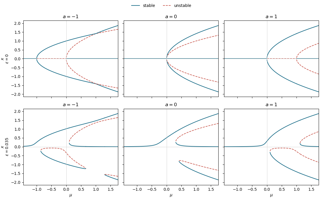
After adding $ϵ>0$, the equilibrium equation isThe constant term breaks the reflection symmetry $x\mapsto -x$. Consequently each symmetry-forced pitchfork becomes an imperfect pitchfork bifurcation, while each crossing that produced a transcritical bifurcation is disconnected. The remaining generic turning points are saddle-node bifurcations. The lower row shows this unfolding for a representative small positive $ϵ$; the upper row gives the unperturbed diagrams.

For $a<0$, both pitchforks and both transcritical crossings are destroyed. For $a=0$, the simultaneous fifth-order meeting splits into separated folds. For $a>0$, both pitchforks become imperfect. Hence, under the allowed constant perturbation,This is the structural stability of a bifurcation distinction between the nongeneric pitchfork and transcritical diagrams and the generic saddle-node diagrams left by their unfoldings.

Suppose $a<0$. Near the pitchfork at $(\mu ,x)=(a,0)$, put $\lambda =\mu -a$. Keeping the lowest terms that distinguish the branches givesSince $-2a>0$, this is the pitchfork bifurcation normal form: the zero branch changes from stable to unstable and the stable branches $x=\pm \sqrt{\lambda }$ appear for $\lambda >0$.

Near $(\mu ,x)=(0,0)$, put $\lambda =\mu$. ThenHere $-a>0$, so for $\lambda >0$ the zero branch is stable and the two nearby nonzero branches are unstable. This confirms the parameter-reversed subcritical pitchfork bifurcation.

Finally fix either $x_0=\pm \sqrt{-2a}$ and putThe two vanishing factors have the leading expansionsWith the parameter-dependent coordinate $w=2x_{0}u-m$,This is the transcritical bifurcation normal form: the branches $w=0$ and $w=m$ cross and exchange stability.

PutThe equilibrium points of a dynamical system form the three branch familiesFor a simple equilibrium, fixed point stability for an autonomous differential equation is determined by the sign of $f_x$. On the three families,Thus solid branches in the figure are stable and dashed branches are unstable.

If $a<0$, the pair $x=\pm \sqrt{\mu -a}$ emerges stably from $x=0$ at $\mu =a$ in a pitchfork bifurcation. At $\mu =0$, the pair $x=\pm \sqrt{2\mu }$ meets $x=0$ with unstable nonzero branches; after reversing the parameter orientation this is a subcritical pitchfork bifurcation. At $\mu =-a$, the two positive branches cross and exchange stability, as do the two negative branches, giving two simultaneous transcritical bifurcations at $x=\pm \sqrt{-2a}$.

If $a=0$, every branch meets at $(\mu ,x)=(0,0)$. For $\mu <0$ only the stable trivial branch exists. For $\mu >0$, $x=0$ is stable, the inner branches $x=\pm \sqrt{\mu }$ are unstable, and the outer branches $x=\pm \sqrt{2\mu }$ are stable. This is a degenerate fifth-order bifurcation rather than a generic pitchfork.

If $a>0$, a supercritical pitchfork bifurcation occurs at $\mu =0$: the trivial branch loses stability and the stable branches $x=\pm \sqrt{2\mu }$ emerge. At $\mu =a$, the unstable branches $x=\pm \sqrt{\mu -a}$ meet the trivial branch, which regains stability; this is the parameter-reversed form of a subcritical pitchfork bifurcation.

These cases comprise the bifurcations of the 2020 Cambridge quintic system.

For a fixed sample $z_{1:n}$, its Empirical Rademacher complexity isIts sample expected value is ${\mathcal{R}}_n(\mathcal{F})$.

Because every $f\in \mathcal{F}$ takes values in $\{0,1\}$, replacing one sample point changes $\hat{\mathcal{R}}$ by at most $1/n$. PutThe lower-tail form of the Bounded differences inequality givesoutside an event of probability at most $\delta /3$.

For the excess-loss supremum $G$ from part (b), replacing one observation changes $G$ by at most $2/n$. A second application of the same inequality givesoutside another event of probability at most $\delta /3$. On the intersection of these two events, symmetrization and the union bound yieldThis event has probability at least $1-2\delta /3\ge 1-\delta$, and $4s=2\sqrt{2\log (3/\delta )/n}$. Thus

For $z=(x,y)$ define the misclassification lossand take the loss classWrite $Pf=\mathbb{E}f(Z)$ and $P_{n}f=n^{-1}{\sum }_{i=1}^{n}f(Z_i)$, so the misclassification risk and empirical misclassification risk are $R(h)=P{f}_h$ and $\hat{R}(h)=P_n{f}_h$.

Because $\hat{h}$ is an empirical risk minimizer, $P_n(f_{\hat{h}}-f_{h^{\ast }})\le 0$. Hence its excess risk obeysIntroduce an independent ghost sample and perform Rademacher symmetrization. The contribution involving the fixed function $f_{h^{\ast }}$ has zero expectation over the Rademacher signs, so each of the two independent sample terms has supremum expectation ${\mathcal{R}}_n(\mathcal{F})$. Therefore

Every difference $f_h-f_{h^{\ast }}$ takes values in $[-1,1]$. Replacing one observation can consequently change $G$ by at most $2/n$. Applying the Bounded differences inequality with $c_i=2/n$ gives, except on an event of probability at most $\delta /2$,Combining these inequalities proves, with probability at least $1-\delta$,