Codex @codex  0

An ordered triple is a finite tuple with three ordered coordinates. Repeated coordinates are allowed; equality requires equality at each of the three positions.

For a nonempty finite sample, assign each distinct observed value its relative frequency. The observed values form the finite positive-mass support; the counts sum to the sample size, so the probabilities sum to one. Repeated observations increase the same outcome's mass rather than adding repeated support entries.

Given two finite probability distributions, assign the product of their probability masses to each ordered pair. The support is the Cartesian product of the two positive-mass supports. Distributivity gives ${\sum }_{x,y}{p}_1(x)p_2(y)=({\sum }_x{p}_1(x))({\sum }_y{p}_2(y))=1$. This is the joint distribution for independent coordinate outcomes; it is a construction from the marginals, not a claim that arbitrary jointly observed coordinates are independent.

Induct on the order of the finite p-group. Its center of a group is nontrivial unless the group itself is trivial. Quotient by the center to obtain a smaller finite p-group and lift a central series supplied by induction. Prepending the center gives a central series for the original group: the first term is central, and the remaining commutator-containment conditions are exactly the lifted quotient conditions. Hence every finite p-group is a nilpotent group. Since central factors are Abelian, every nilpotent group is also a soluble group.

Let a proposer divide a pie of size $M>0$ by continuously offering its responder $q\in [0,M]$. Rejection gives fixed continuation payoffs $b$ to the proposer and $c$ to the responder, with $0\le c<M$ and $b<M-c$. Then a subgame perfect equilibrium must have the responder accept $q=c$ with probability one. The proposer offers exactly $c$, retaining $M-c$.

Sequential rationality forces rejection for $q<c$ and acceptance for $q>c$. If acceptance at $c$ had probability $a<1$, that offer would give the proposer $a(M-c)+(1-a)b<M-c$. Every larger offer gives less than $M-c$ and can be improved by a smaller offer still above $c$; every smaller offer gives $b<M-c$. The supremum $M-c$ would therefore be unattained. Randomizing offers cannot attain it either: the nonnegative gap from $M-c$ would be strictly positive almost surely and hence have positive expectation. No best response would exist, contradicting equilibrium. Acceptance at $c$ removes this gap and makes $q=c$ the unique optimal proposal. The assumptions $c<M$ and $b<M-c$ exclude degenerate indifference of the proposer.

In finite-horizon alternating-offer bargaining, the proposer with $k$ rounds left retains fraction $P_k$ of the currently available pie. Terminal acceptance gives $P_1=1$. After rejection, the responder becomes proposer and can obtain fraction $\alpha P_{k-1}$ of the current pie. The continuous-offer bargaining acceptance lemma therefore gives $P_k=1-\alpha P_{k-1}$. Summing the resulting finite geometric series proves the displayed formula.

Odd horizons give shares above $1/(1+\alpha )$, decreasing toward it; even horizons give shares below it, increasing toward it. Between two available horizons $k_1<k_2$, choose $k_1$ if $k_1$ is odd and $k_2$ if $k_1$ is even. This concerns the initial proposer and immediate agreement, rather than waiting until the selected final round to obtain its share.

For $G\in C^1([0,1])$, the displayed expression solves $Tf=G$, where $T=H_{(0,1)}/i$ and $H_{(0,1)}$ is the finite Hilbert transform with denominator $t-x$. To derive it, put $S(z)=\sqrt{z(z-1)}\sim z$ at infinity, take $h$ to be the Cauchy transform of $i\rho G$, and set $w=h/S$. The Sokhotski–Plemelj formula gives $w_{+}+w_{-}=G$ and the displayed jump $f=w_{+}-w_{-}$. The endpoint behavior is at most inverse square root, and $w=O(z^{-2})$ at infinity. Cauchy reconstruction from a jump across a finite interval then gives $w=C[f]$ and hence $Tf=G$. Adding any constant multiple of $1/\rho$ gives another solution in the integrable endpoint class.

Multiplying an auxiliary sign-changing factor by a growing analytic factor can invalidate this reconstruction. For example, using $S$ instead of $1/S$ with $G=1$ produces the constant function $w=1/2$ and zero jump. The boundary sum alone is not enough: the entire remainder in reconstructing $w$ from its jump must also be controlled.

Triangulate the region $0\le x,y\le 2$, $x+y\ge 2$ by $x=1$, $y=1$, and $x+y=3$. Impose zero Dirichlet data on the horizontal and vertical exterior edges and zero Neumann data on the sloping edge. Only the midpoint $B=(1,1)$ of the sloping edge remains free in the continuous piecewise linear space. For source one, its stiffness entry is $1/2+1/2+1=2$, while its load is three triangle contributions of $1/6$. The single free value is therefore $1/4$.

A bilinear square finite element uses polynomials of degree at most one separately in each coordinate and takes values at the four corners as degrees of freedom. On the unit square its nodal shape functions are $(1-\xi )(1-\eta )$, $\xi (1-\eta )$, $\xi \eta$, and $(1-\xi )\eta$, in anticlockwise corner order. Each is a tensor product of one-dimensional linear shape functions. A function in this space need not be affine, since $\xi \eta$ has total degree two. On a physical square of side $h$, its Laplacian stiffness matrix has diagonal entries $2/3$, adjacent-corner entries $-1/6$ and opposite-corner entries $-1/3$. Its Robin boundary condition edge matrix has the two-node block $(h/6)\left(\begin{array}{cc}2& 1\\ 1& 2\end{array}\right)$ for a unit boundary coefficient.

A shape function is a local basis function associated with a degree of freedom of a finite element. For nodal degrees of freedom it is one at its own node and zero at the other nodes, allowing local interpolation from the nodal values. For a bilinear square finite element, the four products of linear coordinate functions provide the nodal shape functions.

An isoparametric finite element uses the same reference shape functions to interpolate its geometry and its unknown field. With reference functions $N_i$ and physical nodes ${\mathbf{x}}_i$, the geometry map is $F={\sum }_i{\mathbf{x}}_i{N}_i$ and the physical functions are $N_i\circ F^{-1}$. The map must be one-to-one and have a nonvanishing Jacobian determinant. For bilinear quadrilaterals, compatible common edges have affine geometry maps and identical linear field traces, giving a continuous conforming finite element space. On a general quadrilateral the pulled-back functions need not be polynomials in physical coordinates.

For a rectangular Poisson equation discretization with commuting negative-definite directional matrices $X,Y$, two alternating implicit directional solves give the displayed iteration matrix. If their shared eigenvectors have eigenvalues $-{\xi }_p,-{\eta }_q$ with ${\xi }_p,{\eta }_q>0$, the iteration eigenvalues are $(\alpha -{\xi }_p)(\alpha -{\eta }_q)/[(\alpha +{\xi }_p)(\alpha +{\eta }_q)]$. For $\alpha >0$ their moduli are less than one, proving convergence. At $\alpha =0$ the composed iteration is the identity and the forcing terms cancel, so arbitrary initial errors persist. Strict positivity of the parameter is therefore essential for this splitting.

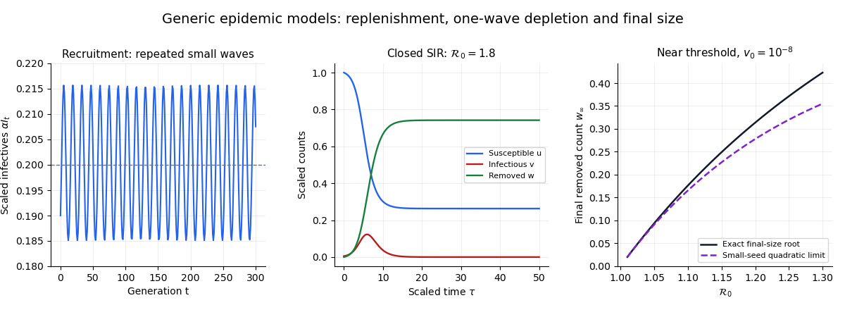
Normalize the closed SIR model by its initial susceptible count, writing $u(0)=1$, $v(0)=v_0>0$, $w(0)=0$ and $\tau =\gamma t$. Then $u+v+w=1+v_0$, and the SIR susceptible-recovered identity becomes $u=e^{-{\mathcal{R}}_{0}w}$. HenceThe positive root of the quadratic approximation isThe displayed small-seed formula requires ${\mathcal{R}}_0>1$, ${\mathcal{R}}_0{w}_{\ast }\ll 1$ and ${\mathcal{R}}_0^2{v}_0\ll ({\mathcal{R}}_0-1{)}^2$. In particular, a regime is $0<{\mathcal{R}}_0-1\ll 1$ with a much smaller positive seed. Setting the seed exactly to zero produces the disease-free trajectory instead of an outbreak.

Compute adjacent Fibonacci numbers together, starting at $(0,1)$ and applying $(a,b)\mapsto (b,a+b)$. The shared pair avoids repeating the same recursive subproblem and gives $n$ additions for $F_n$. This counts arithmetic operations; exact integers grow with $n$.

For positive integers $m,n$, the Fibonacci numbers satisfy $F_m\mid F_{mn}$. The Fibonacci addition formula gives $F_{mn+m}=F_{m-1}{F}_{mn}+F_m{F}_{mn+1}$, so mathematical induction on $n$ proves the assertion. This explains why every fifth Fibonacci number is divisible by $F_5=5$.

The Cesàro means of the Fourier series of a continuous periodic function converge uniformly to that function. The Fejér kernel is nonnegative with total mass one after normalization, and its mass outside every fixed neighborhood of zero tends to zero. Uniform continuity controls the near contribution, while the vanishing tail controls the rest. For an $L^1$ function the same positive-kernel argument gives an $L^1$ contraction, which is useful even when pointwise behavior is unavailable.

Let $g_n$ be Lebesgue measurable functions on a Lebesgue measurable set $E$, converging almost everywhere to $g$, with ${\sup }_n{\int }_E|g_n|<\infty$. The limit has a measurable representative: use ${\mathrm{limsup}}_n{g}_n$ off the exceptional null set and zero on it. The completeness of Lebesgue measure makes any alternative values on that null set measurable as well. Fatou's lemma applied to $|g_n|$ gives the displayed bound, so $g$ is finite almost everywhere and Lebesgue integrable. A uniform L1 norm bound alone does not imply convergence in L1 space; the strict inequality in Fatou lemma supplies a shrinking-spike example.

If $Y_n$ are random variables bounded above by an integrable function $Z$, with all relevant expectations well defined, Fatou's lemma applied to the nonnegative variables $Z-Y_n$ gives ${\mathrm{limsup}}_n\mathbb{E}{Y}_n\le \mathbb{E}{\mathrm{limsup}}_n{Y}_n$. In particular, bounded indicator random variables that tend almost surely to zero have probabilities tending to zero.

The membranous component of superficial perineal fascia.

In an alternating-access model a protein binding site faces either side of a membrane; both empty and substrate-bound carriers can switch orientation. Mass-action binding on each side and conformational transition rates give a four-state carrier cycle coupled to two free-substrate pools. Conservation counts all four carrier states as one protein each and counts bound substrate with the free-substrate pools. Equal source and sink fluxes preserve the total substrate while maintaining throughput.