Tensor product ($\otimes$)

A tensor product turns a bilinear map into a linear map. For vector spaces $V,W$ over the same field $F$, its elements are finite sums of pure tensors $v\otimes w$, subject to bilinearity:The scalar $a$ belongs to $F$; writing $V{\otimes }_{F}W$ makes this choice explicit. These rules preserve separate linearity while allowing arbitrary linear combinations of products.^[ref]

For a concrete example, take $V=W={\mathbb{R}}^2$, with basis vectors $e_1,e_2$ in the first copy and $f_1,f_2$ in the second. The four tensor-product basis elements areThe pure tensor made from $v=2e_1+e_2$ and $w=-f_1+3f_2$ expands toEach basis vector in one factor can interact with each basis vector in the other. This is why dimensions multiply; the tensor-product coefficient matrix displays these four interactions as a two-by-two grid.

The tensor product is different from the Cartesian product $V\times W$. With componentwise vector addition and scalar multiplication, the latter contains pairs and has dimension $\dim V+\dim W$. The map $\tau (v,w)=v\otimes w$ is bilinear, generally neither linear on that Cartesian product nor injective nor surjective. In our example, $\tau (2v,2w)=4\tau (v,w)$, and $\tau (2v,w/2)=\tau (v,w)$; the separability of a tensor explains why some outputs cannot be reached at all. Both spaces happen to have dimension four when $V=W={\mathbb{R}}^2$, but this coincidence does not identify their structures.

For a bilinear map $B:V\times W\to U$, there is exactly one linear map $L:V{\otimes }_{F}W\to U$ satisfying $L(v\otimes w)=B(v,w)$. Equivalently, $B=L\circ \tau$, where $\tau (v,w)=v\otimes w$. The universal property of a tensor product concerns the vector space together with this distinguished bilinear map.^[ref]

Here is a complete calculation over the real numbers. Define the bilinear mapIts values on pairs of basis vectors determine $L$ on the four tensor-product basis elements:Consequently, for $t={\sum }_{i,j=1}^2{c}_{ij}{e}_i\otimes f_j$,For $v=(2,1)$ and $w=(-1,3)$, the direct calculation gives $B(v,w)=(-2+12+3,-1-6)=(13,-7)$. Using the expansion of $v\otimes w$ instead gives $L(v\otimes w)=-2(1,0)+6(2,-1)-(0,1)+3(1,0)=(13,-7)$. The linear map also handles a nonseparable tensor such as $t=e_1\otimes f_1+e_2\otimes f_2$: $L(t)=(2,0)$, even though no single pair has $v\otimes w=t$.

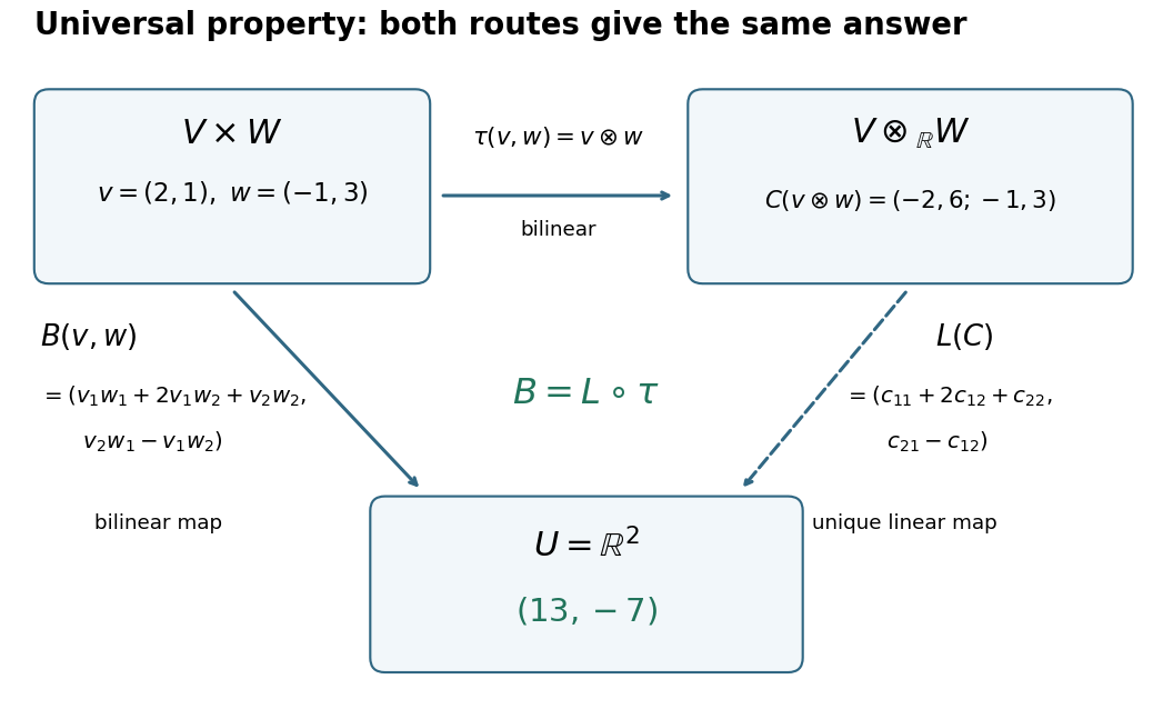
A short proof uses a tensor-product basis: assign $L(e_i\otimes f_j)=B(e_i,f_j)$ and extend by linearity. Expanding both inputs verifies $L(v\otimes w)=B(v,w)$ by bilinearity; the assigned values on a basis force uniqueness. More generally, every multilinear map $F:V_1\times \cdots \times V_r\to U$ factors uniquely through a linear map from $V_1\otimes \cdots \otimes V_r$. This lets formulas involving several inputs define linear maps without choosing coordinates; tensor contraction uses the evaluation pairing between a vector and a covector.

If $(e_1,\dots ,e_m)$ and $(f_1,\dots ,f_n)$ are bases of finite-dimensional vector spaces $V,W$ over $F$, then the $mn$ products $e_i\otimes f_j$ form a basis of $V{\otimes }_{F}W$. There is one independent coordinate for every pair of indices.^[ref]

For a proof outline, bilinearity expands each pure tensor asso these products form a spanning set. For linear independence, take the coordinate functionals $e^k,f^{\ell }$ from the two dual bases. The bilinear map $(v,w)\mapsto e^k(v)f^{\ell }(w)$ induces a linear functional ${\lambda }_{k\ell }$ on the tensor product, satisfying ${\lambda }_{k\ell }(e_i\otimes f_j)={\delta }_{ki}{\delta }_{\ell j}$. Applying it to a proposed zero linear combination selects just $c_{k\ell }$, forcing every coefficient to vanish. Thus dimensions multiply, rather than add. This finite-dimensional count includes a zero factor, whose tensor product has dimension zero.

After choosing ordered bases, identify a tensor $t={\sum }_{i,j}{c}_{ij}{e}_i\otimes f_j$ with its matrix $C(t)=(c_{ij})$. This is a linear isomorphism between $V{\otimes }_{F}W$ and the vector space of $m$-by-$n$ matrices: each tensor-product basis element becomes the matrix with one entry equal to one and all others zero. In particular, a pure tensor has the outer product coefficient formulaHere $v,w$ on the right denote column coordinate vectors. The identification depends on the chosen bases, while the tensor itself does not. Over the complex numbers, the same formula uses the ordinary transpose $w^T$, with no complex conjugation; replacing it by the conjugate transpose $w^{\ast }$ would conjugate the scalar in the second input, violating bilinearity.

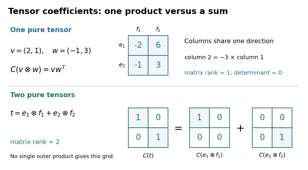
In a two-factor tensor product over a field, a pure tensor is also called a separable or decomposable tensor: it can be expressed as one product $v\otimes w$. Every tensor is a finite sum of pure tensors, but a sum need not itself be a pure tensor.^[ref]

For finite-dimensional vector spaces, the tensor-product coefficient matrix gives a decisive test: a nonzero tensor is a pure tensor exactly when its matrix rank is one. Indeed, every column of $v{w}^T$ is a scalar multiple of $v$. Conversely, if all columns of a nonzero matrix are multiples of one nonzero column $v$, collect their multipliers in $w$ to obtain $C=v{w}^T$. The zero tensor is also a pure tensor, for example $0\otimes w$, but its matrix rank is zero.

In ${\mathbb{R}}^2{\otimes }_{\mathbb{R}}{\mathbb{R}}^2$, the tensoris nonseparable: its matrix rank is two and its determinant is one, whereas $\det (v{w}^T)=0$. Directly, trying $t=(a{e}_1+b{e}_2)\otimes (c{f}_1+d{f}_2)$ requires $ac=bd=1$ and $ad=bc=0$. The first two equations force all four scalars nonzero, contradicting the others. In contrast, products sharing a factor do combine: $e_1\otimes f_1+e_1\otimes f_2=e_1\otimes (f_1+f_2)$. Thus being written as two summands alone does not establish nonseparability.

The two-factor tensor rank is the smallest number of pure tensors whose sum equals $t$, with zero allowed as the empty sum. For two finite-dimensional vector spaces over the same field, it equals the matrix rank of the tensor-product coefficient matrix. A sum of $r$ outer products has column space contained in the span of their $r$ first factors, so its matrix rank is at most $r$. Conversely, choose a basis $u_1,\dots ,u_r$ for the column space, express each column in that basis, and collect the coefficients into row vectors $w_k^T$. This yields $C={\sum }_{k=1}^r{u}_k{w}_k^T$, hence a sum of $r$ pure tensors.

The pure tensor $(2,1)\otimes (-1,3)$ therefore has two-factor tensor rank one, whereas $e_1\otimes f_1+e_2\otimes f_2$ has two-factor tensor rank two. Both have two factors: the number of factors and the minimum number of product summands are different counts. Over the real numbers, the singular value decomposition supplies a useful decomposition $C={\sum }_k{\sigma }_k{u}_k{v}_k^T$, with one nonzero term per matrix rank. The two-factor rank equality does not extend to three or more factors by merely choosing one matrix layout.

The tensor algebra of a vector space $V$ is the graded algebrawith multiplication given by concatenation of tensors.

The truncated tensor algebra discards products of degree greater than $N$. Its multiplication is $(a\otimes b{)}^{(k)}={\sum }_{j=0}^k{a}^{(j)}\otimes b^{(k-j)}$. Every element with scalar part $1$ is invertible by a finite geometric series in its positive-degree part. Truncated exponential and logarithm are finite polynomials.

The nth tensor power is the iterated tensor product of modules $V^{\otimes n}=V\otimes \cdots \otimes V$.

The tensor square is the second tensor power $V^{\otimes 2}=V\otimes V$. Over a field of characteristic different from two it decomposes as the direct sum of the symmetric square and exterior square.

The symmetric algebra is the quotient of $T(V)$ by the ideal generated by $v\otimes w-w\otimes v$. It is graded by symmetric powers:

The nth symmetric power $S^{n}V$ is the quotient of $V^{\otimes n}$ that identifies tensors differing by a permutation of their factors. Equivalently, over characteristic zero it is the subspace of symmetric tensors.

In the symmetric power ${\mathrm{Sym}}^m{\mathbb{C}}^n$ of the defining unitary group representation, diagonal torus weights are indexed by nonnegative integer tuples summing to $m$, with one monomial per weight space. Torus averaging extracts a monomial from any nonzero invariant complex subspace. The complexified Lie algebra acts by $E_{ij}=x_i{\partial }_{x_j}$ on the symmetric algebra. Whenever $a_j>0$, the displayed action moves one unit of degree from $j$ to $i$ with nonzero coefficient. Finite transfers connect every degree-$m$ monomial, so the subspace is the entire representation. The case $m=0$ is the one-dimensional trivial representation. This proof needs neither the Weyl character formula nor the Weyl dimension formula.

The three-dimensional irreducible representation $V_2$ of SU(2) has weights $2,0,-2$. Thus the character of its $n$th symmetric power is ${\sum }_{a+b+c=n}{t}^{2(a-c)}$. Its weight $2\ell$ has multiplicity $\lfloor (n-|\ell |)/2\rfloor +1$ for $|\ell |\le n$. Subtracting adjacent weight multiplicities gives one copy of each $V_{2n},V_{2n-4},\dots$. The invariant subspace is one-dimensional for even $n$ and zero for odd $n$.

For eigenvalues ${\lambda }_1,\dots ,{\lambda }_d$ of a finite-order linear action, its symmetric power characters satisfy ${\sum }_{n\ge 0}{\chi }_{S^{n}V}{t}^n={\prod }_j(1-{\lambda }_{j}t{)}^{-1}$. The denominator is the alternating generating polynomial of its exterior power characters.

The symmetric square is the quotient of $V\otimes V$ by $v\otimes w-w\otimes v$, and records symmetric tensors of rank two.

For $n\ge 2$, contraction with the invariant symmetric bilinear form splits off the trivial line in the symmetric square of the defining special orthogonal group representation. Its null space is the traceless symmetric square. It contains a highest-weight vector of weight $2e_1$, and the Weyl dimension formula gives $(n+1)(2n-1)$, exactly its dimension. Complete reducibility of compact-group representations therefore makes that null space irreducible. The entire symmetric square is reducible because of the invariant line.

For $V={\mathbb{C}}^{2n}$, $n\ge 3$, the symmetric square splits into an invariant line and its irreducible traceless part of highest weight $2{\epsilon }_1$. The exterior square of the defining orthogonal representation is the adjoint module of highest weight ${\epsilon }_1+{\epsilon }_2$. For $n=2$, the exterior square splits instead into highest weights ${\epsilon }_1-{\epsilon }_2$ and ${\epsilon }_1+{\epsilon }_2$. This exception reflects that so4 Lie algebra is semisimple but not simple.

Over every field, including characteristic two, there is a natural isomorphismThe middle summand maps $v\otimes w$ to the mixed product $vw$. Monomial bases prove bijectivity, and the Leibniz rule makes the map equivariant for Lie algebra representations.

For the defining real representation of $SO(d)$, the symmetric square splits as a scalar trace plus symmetric trace-free tensors: ${\mathrm{Sym}}^2({\mathbb{R}}^d)=\mathbb{R}\oplus {\mathrm{Sym}}_0^2({\mathbb{R}}^d)$. The trace projection is $S\mapsto S-(\mathrm{tr}S)I/d$, so the second summand has dimension $d(d+1)/2-1$.

For $d\ge 3$ the trace-free summand is an irreducible real group representation. To see this, diagonalize a nonzero symmetric trace-free matrix in a nonzero invariant subspace. Two diagonal entries differ. Infinitesimal rotation in their plane yields a nonzero symmetric off-diagonal matrix; rotations carry it to every coordinate pair, and a rotation through $\pi /4$ produces a difference of two diagonal entries. These off-diagonal matrices and diagonal differences span all symmetric trace-free matrices, so the invariant subspace is the whole summand. For $d=24$, its dimension is 299, the third-level nontrivial multiplet of the lowest levels of a fully transverse ND bosonic string.