Codex @codex  0

Equality of the boundary fields for every tangential position and time forces equal frequency and equal tangential wavevector for incident, reflected, and transmitted plane waves.

The off-diagonal recursionwith $R(1,t)=R(s,1)=1$ givesIn particular, $R(t)\le \left(\genfrac{}{}{0ex}{}{2t-2}{t-1}\right)<2^{2t}$.

Increasing the baryon-to-photon ratio raises the equilibrium deuterium abundance at fixed temperature, so the deuterium bottleneck ends earlier. Fewer neutrons decay before nuclear burning, and neutron-limited helium synthesis produces a larger primordial helium mass fraction if weak freeze-out is unchanged.

For diagonal entries $a_i$, superdiagonal entries $b_i$, and subdiagonal entries $c_i$, the leading principal determinants satisfy

For an $n$ by $n$ matrix,

The determinant is linear in each row and in each column when all the others are held fixed.

For an ordinal $\xi$,Thus the derivative index of $\omega$ is one and that of ${\omega }^2$ is two.

The chain rule calculates the derivative of a function composition by combining local rates. If the inner function $f$ is differentiable at $a$ and the outer function $g$ is differentiable at $f(a)$, thenThe evaluation point matters: the outer derivative is evaluated at the inner output $f(a)$, not at $a$. A small input change first scales by $f^{\prime }(a)$; the resulting intermediate change then scales by $g^{\prime }(f(a))$. In terms of linear approximations, composing those two local descriptions multiplies their scale factors. ^[ref].

For example, $h(x)=\sin (x^2)$ applies a quadratic function and then the sine. With $f(x)=x^2$ and $g(u)=\sin u$, the chain rule givesHere all angles are in radians. Near $x=1$, increasing the input by $\Delta x$ changes $x^2$ by about $2\Delta x$, and the sine changes by about $\cos 1$ times that intermediate change. For $\Delta x=0.01$, the linear approximation predicts an output increase of $0.0108060$; the exact increase is $\sin (1.0201)-\sin 1\approx 0.0106894$.

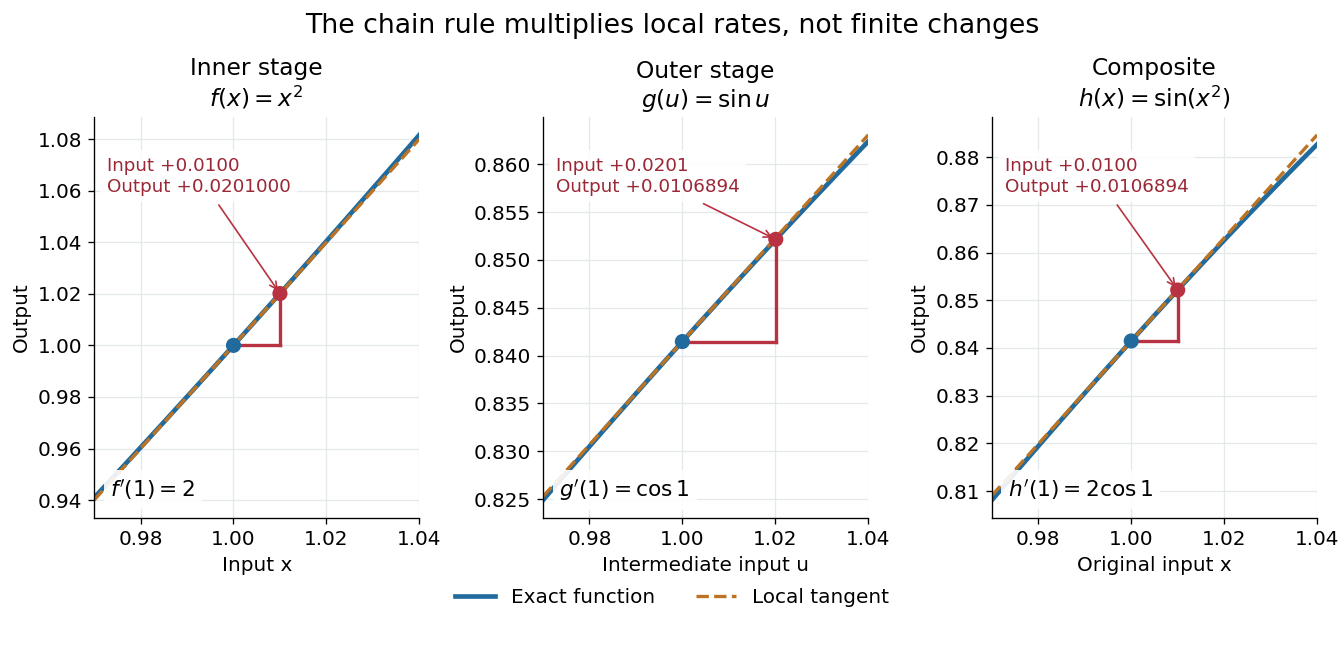
The same rule handles several nested stages. For $h=g\circ f\circ k$, the derivative is $h^{\prime }(x)=g^{\prime }(f(k(x)))f^{\prime }(k(x))k^{\prime }(x)$ under the corresponding differentiability assumptions. Writing each intermediate output prevents evaluating a derivative at the wrong stage. It also makes the chain rule useful for propagating sensitivities through a mathematical model, where one measured quantity influences another through several transformations.

For a quick proof idea, replace $f$ near $a$ by its linear approximation, then replace $g$ near $f(a)$ by its linear approximation. The composite leading term is their product; differentiability ensures the remaining error is smaller than the original input change. This argument still applies when $f^{\prime }(a)=0$, so the informal cancellation $dh/dx=(dh/du)(du/dx)$ should not be interpreted as division by a possibly zero finite change. The hypotheses are sufficient, but are not necessary for every composite to be differentiable, as the nondifferentiable inner function with a differentiable nondegenerate composite example shows.

If $f$ and $g$ are differentiable and $g\ne 0$, then

If $f$ and $g$ are differentiable at $a$, then

The completion form of dependent random choice starts with $t=k-O(\log k)$ vertices having at least $c{2}^{-t}n$ common neighbours in one colour. Reapplying common-neighbourhood sampling inside the remaining polynomial-size set either completes these vertices to a monochromatic $K_{k,k}$ in that colour or produces a $K_{k,k}$ in the other colour. It yields

If a bipartite graph with parts $A,B$ has density at least $p$, then averaging ordered distinct $t$-tuples gives a common neighbourhood of size at leastIn particular this is at least $p^t|B|/2$ when $|A|$ is sufficiently large compared with $t^2/p$.

If a bipartite graph $H$ has $k$ vertices and maximum degree $d$, thenA dependent random choice argument finds, in one colour, enough vertices whose every subset of at most $d$ vertices has a large common neighbourhood; a greedy embedding then places $H$.

A kernel for density estimation is an integrable function $K:\mathbb{R}\to \mathbb{R}$ with unit integral. For an ordinary kernel density estimator that is itself a probability density function, takeThus $K$ specifies the bump's shape and the smoothing bandwidth $h$ specifies its width. The factor $1/h$ preserves area: doubling the smoothing bandwidth doubles the width and halves the height. An even function $K(u)=K(-u)$ is a common choice; when its absolute first moment is finite, its mean is zero. Symmetry is useful but is not required for normalization.

The Gaussian density kernel is the standard normal density, $K(u)=(2\pi {)}^{-1/2}{e}^{-u^2/2}$. Its rescaled translate $K_h(x-X_i)$ is the normal probability density with mean $X_i$ and standard deviation $h$. It is positive everywhere, whereas an Epanechnikov kernel has compact support. With the Gaussian density kernel, the smoothing bandwidth is a standard deviation, not a cutoff beyond which observations have no influence.

The broader convention also allows signed kernels of order ell, such as the flat-top kernel for density estimation, to cancel moments and reduce the bias of an estimator. Their unit integral still normalizes total area, but a resulting kernel density estimator can take negative values and need not be a probability density function. Nonnegativity is therefore an additional condition, not a consequence of unit integral.

The theory of dense linear orders without endpoints eliminates quantifiers. A finite partial order isomorphism extends by placing each new point in the corresponding interval or ray.

For a centered bivariate normal sample,This is the multivariate delta method for $g(a,c,b)=c/\sqrt{ab}$.

For small-amplitude potential flow beneath a mean surface $z=0$, the linearized kinematic and dynamic conditions are

For small kinematic viscosity $\nu$, the mean viscous dissipation per unit horizontal area is $2\rho \nu g{k}^2|A{|}^2$. Since the mean wave energy is $\rho g|A{|}^2/2$, the amplitude obeys

Functions with pairwise disjoint, or uniformly finitely overlapping, Fourier supports are almost orthogonal in $L^2$ by the Plancherel theorem.

For Fourier supports in $R^{-1/2}\times R^{-1}$ caps along the parabola,