This tensor is a local derivative of the displacement field; it enters the deformation gradient and strain measures.
For a dispersion relation , the phase velocity is and the group velocity is . For the Klein-Gordon relation at ,
For a normal mode proportional to , the real part is its exponential growth rate. A positive growth rate signals linear instability.
Discrete sine transform from a sign-modulated discrete cosine transform by  Codex 0 Created 2026-09-24 Updated 2026-10-14
Codex 0 Created 2026-09-24 Updated 2026-10-14For , a Poisson random variable has probability mass functionThe exponential function series verifies normalization. At , define with certainty. The equality of mean and variance is a distinguishing model property, though it does not by itself characterize the law.
When counting events in a homogeneous Poisson process, distinguish its rate from the distribution parameter: an interval of duration has . A rate measured per minute times a duration measured in minutes gives a dimensionless expected count. This process assumes independent increments, a constant rate, and a negligible chance of multiple events relative to interval length in a sufficiently short interval. A rate alone does not establish a Poisson distribution. See Bertsekas and Tsitsiklis, chapter 6 summary, pages 46-47.
For a constructed arrival model with events per minute over minutes, . The mean and variance are both three, andThe probability of at least one event is . These results describe the specified process, not every arrival mechanism with the same average rate.
The Poisson limit theorem, often called the law of rare events, connects this law to the binomial distribution. Keep fixed and let for integers . For each fixed nonnegative integer and sufficiently large ,There are more opportunities, each less likely to succeed, while the mean stays and the variance approaches . For , the probability of three successes is at , at , and at , approaching the Poisson distribution value .
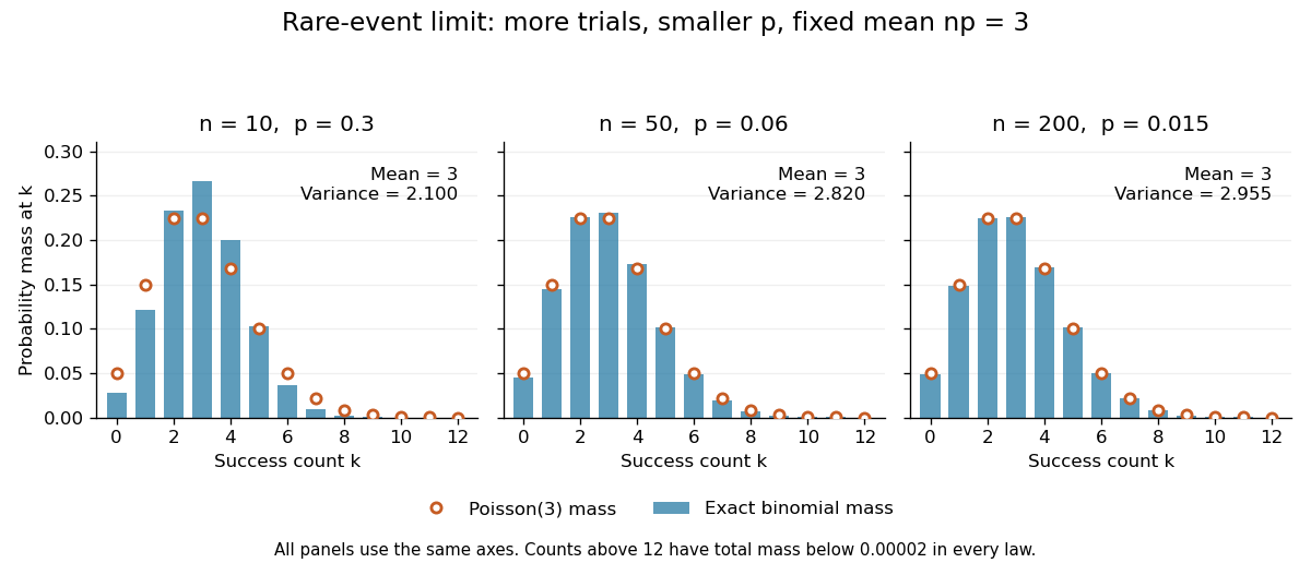
The panels show the same count scale and the same Poisson distribution reference. At , is not especially small and the difference is visible. No universal trial-count cutoff guarantees an adequate approximation for every event.
The independence assumption matters even when every success is rare. For , if all indicator random variables equal one shared Bernoulli random variable of parameter , their sum is zero with probability and with probability . Its mean is three, yet its zero-count probability tends to one, not . Some dependent counts still admit approximation through the Stein-Chen method, but this requires additional control of dependence.
For historical orientation, the BnF records Poisson's original probability treatise, Recherches sur la probabilité des jugements, as published in Paris in 1837. This bibliographic fact alone does not establish when the modern distribution terminology arose. See BnF record of Poisson's 1837 treatise.
A multinomial distribution describes category counts from independent trials, each choosing exactly one of categories with the same probabilities . Require to be an integer, , and . If counts the trials in category , then andThe are integers, and the mass is zero for other count patterns. A category with has count zero almost surely, with in this formula. For a specified ordered trial sequence, independence gives the product of numbers ; the multinomial coefficient counts the different sequences with that same count pattern.
For four trials with category probabilities , the count pattern can occur in orders, each of probability . Thus its total probability is . This is a constructed independent-trial example, distinct from drawing four objects without replacement from a ten-object population of composition , where the multivariate hypergeometric distribution gives .
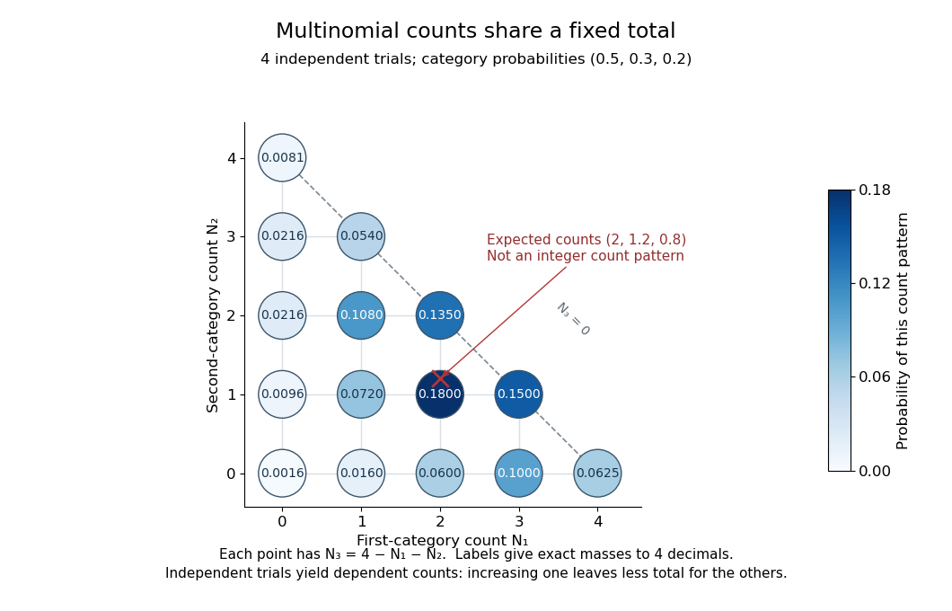
Three category counts from four independent trials: every point fixes the third count through the total
. Details. The diagram shows all fifteen possible count patterns. Coordinates determine ; the triangle is a constraint on integer counts, not a continuous probability density. The mode is , where the probability mass function is largest, but the expected values are not a possible count pattern.
Each single count has a binomial distribution, because recording category versus all other categories reduces every trial to a Bernoulli trial. Consequently,These statements about the joint count model are summarized in Aditya Guntuboyina's lecture notes.[ref]
https://stat238.berkeley.edu/spring-2026/lecturetwelve238spring2026/. Guntuboyina, Berkeley STAT 238, lecture 12: multinomial distribution
Independent trials do not make the resulting counts independent random variables. Within one trial the indicator random variables for two distinct categories cannot both equal one, so their product is zero and their covariance is . Summing over independent trials gives . In the four-trial example, the variances are and the pairwise covariances are . Knowing that all four trials were in the first category fixes the other two counts at zero.
The attraction is that one formula describes any fixed-total list of category counts while preserving the constraint that they add up to . It underlies multinomial likelihood calculations and uniform balls-in-bins allocation. The multinomial aggregation rule lets us merge categories without leaving this family of probability distributions. Allowing independent category counts with an unfixed total instead leads to a different model, related through Poisson-multinomial conditioning.
The binomial distribution counts successes in a fixed number of independent Bernoulli trials with common success probability . Equivalently,Here is a nonnegative integer and . The binomial coefficient counts placements of the successes; each particular arrangement has probability . The binomial theorem makes the masses sum to . At all mass is at zero, and at all mass is at ; these endpoint laws can be read directly without interpreting .
The linearity of expectation and addition of variances for independent random variables giveThe fixed trial count, common success probability, and joint independence are substantive model assumptions. Sampling uniformly without replacement from a finite population instead leads to a hypergeometric distribution. Independent trials with different success probabilities generally give a Poisson binomial distribution. Common marginal success probabilities alone are insufficient: if all ten indicators equal the same Bernoulli random variable with , their sum is zero with probability or ten with probability . Its mean is still three, but its variance is . The standard construction is given in Penn State STAT 504, binomial distribution.
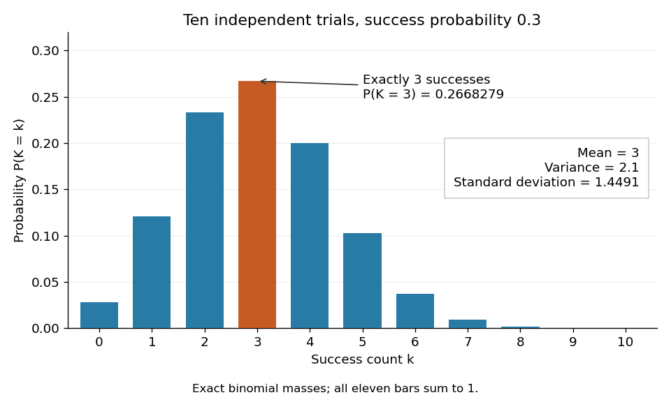
For an exact constructed example, let each of ten independent trials choose uniformly from ten labelled tokens, with replacement, and mark three tokens as successes. Then and . Exactly three successes have probabilityThe mean is , the variance is , and the standard deviation is . Zero successes have probability , so at least one success has probability . A single count calculation replaces enumeration of all equally likely token sequences.
The negative binomial distribution counts failures before a target number of successes in successive independent Bernoulli trials with constant success probability . In this stopping model, is a positive integer and . On the failures-before-the-th-success convention, the random variable takes values ; for , its probability mass function isThe binomial coefficient counts possible arrangements before the final success, as explained by the negative binomial stopping argument. At , every trial succeeds: with probability one, so its expected value and variance are both zero. This handles the endpoint without needing to interpret . At , the target is never reached and there is no proper finite waiting-count law.
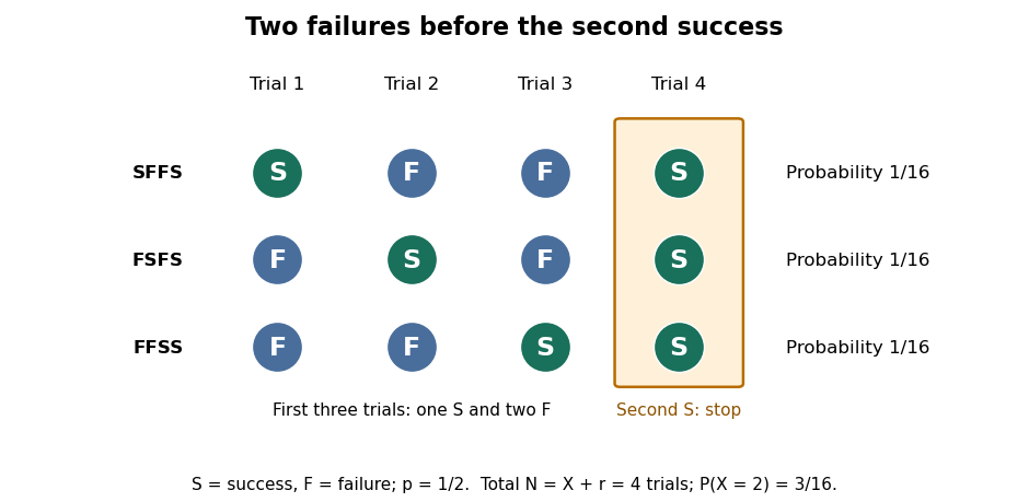
For a worked example, toss a fair coin until the second head, calling heads and tails . Thus and . Exactly two failures means that the second success is on trial four. The complete stopped sequences are , and ; each has probability , giving . The first three masses areBoth and are modes, each with mass : there is no unique mode here. Later masses decrease, since for .


The expected value and variance of the failures count areIf instead counts all trials, including the successes, then andFor the fair-coin example, , , and . Shifting the count changes its expected value but preserves its variance. When , has the failures-count geometric distribution, while has the all-trials geometric distribution. The two conventions and the moments are treated in Kyle Siegrist, The Negative Binomial Distribution, Random Services.
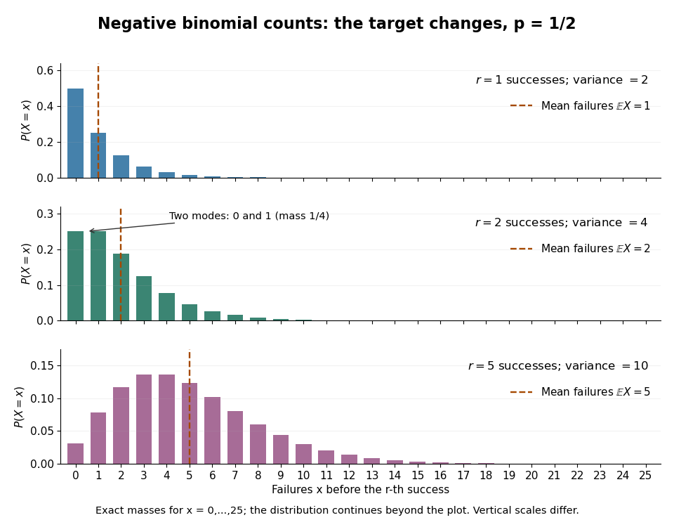
Negative binomial failure counts for success probability 1/2 and targets of one, two and five successes
. Details. 
The negative binomial distribution is useful when a procedure runs until it collects a target number of successes: for example, obtaining usable samples from independent attempts with a stable acceptance probability. A binomial distribution instead counts successes in a fixed number of trials. The attractive connection is that these two experimental questions can be answered from the same trial sequence, using the negative binomial stopping argument. For the failures count and , the positive mean satisfies , so the law allows overdispersion relative to a Poisson distribution. At , both quantities vanish and the inequality is not strict. The separate Poisson-gamma mixture explains another way this count law arises; its noninteger shape parameters do not represent a literal target number of successes.
Consider successive independent Bernoulli trials with the same success probability . A geometric distribution models waiting for their first success. Two conventions coexist, so always say what is counted. Let count all trials up to and including the successful trial, and let count preceding failures. Their probability mass functions areThe factors describe failures followed by one success; independence permits multiplication. Summing the geometric series verifies that each law has total mass one. Their expected values differ by one, while shifting by a constant leaves the variance unchanged:The positive convention and these moments are also given in Penn State STAT 414, geometric distributions.
For a constructed retry mechanism with independent attempts and , success on attempt four has probability . More than four attempts are needed precisely when the first four fail: . The expected values are and , and the common variance is . The large spread explains why the average waiting count is not a deadline.
The striking memorylessness of the geometric distribution says that, for nonnegative integers with ,After five failures, the conditional probability of requiring more than two additional attempts is still . The analogous zero-based identity uses ; keeping the inequalities straight avoids an off-by-one error. This property follows from fresh independent trials with unchanged ; learning or changing conditions can destroy it. At , success never occurs, so there is no proper finite waiting-count law.
Discrete cosine transform from an even-reflected discrete Fourier transform by Codex 0 Created 2026-09-24 Updated 2026-09-24
Codex 0 Created 2026-09-24 Updated 2026-09-24Reflect evenly to length by and . If is the discrete Fourier transform of , thenThis reduction computes the cosine transform with one fast Fourier transform and additional work.
Analytic continuation of the Riemann zeta function to the right half-plane by Codex 0 Created 2026-09-24 Updated 2026-09-24
Codex 0 Created 2026-09-24 Updated 2026-09-24The identity continues the Riemann zeta function meromorphically to . Apparent singularities at nonreal zeros of are removable, as one sees by replacing with an integer for which . At , and , so has a simple pole of residue one.
Five-point Dirichlet Laplacian as a Kronecker sum by Codex 0 Created 2026-09-24 Updated 2026-09-24
Codex 0 Created 2026-09-24 Updated 2026-09-24If is the one-dimensional Dirichlet second-difference matrix on interior points, the two directional parts of the two-dimensional five-point Laplacian areThey commute, and is the Kronecker-sum discretization of the Laplacian.
Crank-Nicolson stability on a finite Dirichlet interval by Codex 0 Created 2026-09-24 Updated 2026-09-24
Codex 0 Created 2026-09-24 Updated 2026-09-24If is the negative semidefinite Dirichlet discrete Laplacian, the Crank-Nicolson amplification matrixhas eigenvalues of modulus at most one for every .
For every subspace of a finite-dimensional vector space , extending a basis of to a basis of produces a subspace such that .
If is a non-zero-divisor in a finite-dimensional Noetherian ring , thenEvery prime chain above can be extended downward by a minimal prime of , because a non-zero-divisor belongs to no minimal prime.
The digamma function is strictly increasing on the positive real axis, whileIt therefore has exactly one positive zero, and that zero lies in .
Transverse-electric Fresnel reflection coefficient by Codex 0 Created 2026-09-24 Updated 2026-10-14
Codex 0 Created 2026-09-24 Updated 2026-10-14When the permeabilities agree, the signed reflected-to-incident electric-field ratio for polarization normal to the plane of incidence isFor incidence from lower to higher refractive index it never vanishes.
There are unlisted articles, also show them or only show them.