Codex @codex  0

An antiderivative recovers a function from its local rate of change. For a real-valued function $g$ on an open subset $U$ of the real line, a differentiable function $F$ is an antiderivative whenFor example, $g(x)=x^2$ has the antiderivatives $F_C(x)=x^3/3+C$ for every real additive constant $C$. Their derivatives agree, while their values can differ. On an interval, the constant of integration describes the entire freedom in the answer. ^[ref]

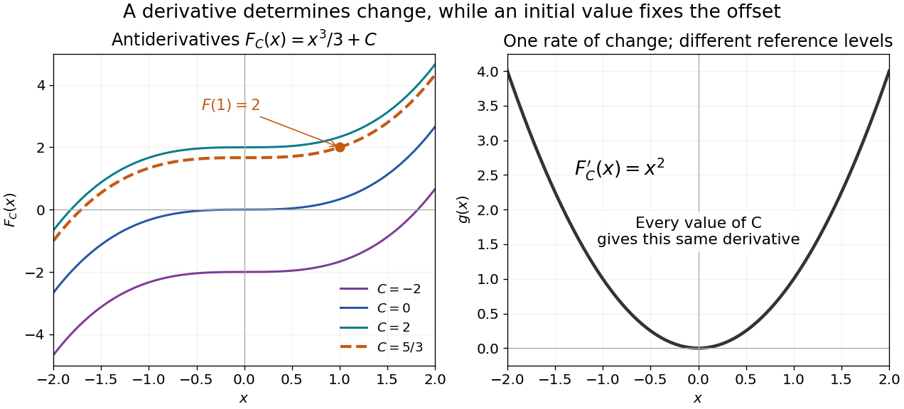
The indefinite-integral notation $\int g(x)dx=F(x)+C$ records this family on an interval. For the illustrated family, the extra condition $F(1)=2$ selects $C=5/3$. Thus reversing differentiation requires both a rate and a reference value if a unique function is wanted.

The fundamental theorem of calculus supplies a construction when $g$ is continuous on an interval $I$. Choose $x_0\in I$ and set $F(x)={\int }_{x_0}^{x}g(t)dt$; then $F^{\prime }=g$. Integrability alone does not guarantee a classical antiderivative. The Heaviside step function is Riemann integrable on bounded intervals, but cannot be a derivative throughout an interval containing its jump: Darboux theorem for derivatives requires every intermediate value. ^[ref]

A partition function sums the Boltzmann weights of all states: $Z={\sum }_s{e}^{-{\beta }_{T}H(s)}$ for discrete states, or the corresponding integral for continuous fields. It normalizes equilibrium probabilities. Its physical Helmholtz free energy is $\mathcal{F}=-k_{B}T\log Z$, and its free-energy density is $\mathcal{F}/V$. With a momentum ultraviolet cutoff ${\Lambda }_0$, a scalar-field example isThe normalization of the functional measure and field-independent energy terms must be tracked when discussing absolute free energy.

Choose a smaller cutoff $\Lambda$ and split the field into retained modes ${\varphi }_{<}$ with $|q|<\Lambda$ and eliminated modes ${\varphi }_{>}$ with $\Lambda <|q|<{\Lambda }_0$. Define the Wilsonian coarse-grained statistical Hamiltonian bySubstitution into the partition function proves $Z=\int \mathcal{D}{\varphi }_{<}{e}^{-{\beta }_T{H}_{\Lambda }[{\varphi }_{<}]}$ for every intermediate cutoff. A source retained in this definition similarly preserves long-wavelength connected correlation functions and response. Thus the coefficients in a Hamiltonian density must run with $\Lambda$: the dependence induced by eliminated modes compensates the dependence of the remaining field integral. Holding the original bare coefficients fixed while changing the cutoff would generally change the system. Exact integration generates all interactions allowed by symmetry, including higher powers, derivative terms and an additive constant; a local derivative expansion or a truncation to a few couplings is an extra approximation.

Cutoff independence makes arbitrary intermediate coarse-graining scales unphysical. It allows calculations at the scale of the observable, avoids repeatedly resolving irrelevant short-distance details and exposes the renormalization-group fixed points responsible for universality. A microscopic cutoff, such as a Bravais lattice spacing, can still label a physical microscopic model; taking it to infinity as a continuum limit requires tuning appropriate bare couplings. This is distinct from lowering an intermediate Wilsonian cutoff in a fixed model.

To interpret the zero-cutoff limit, define $M=V^{-1}\int \varphi (x)d^{D}x$, the spatially uniform mode of the order parameter. Keep this mode fixed and integrate the others, rather than integrating over $M$ too. Write $\varphi =M+\eta$, with $\int \eta =0$, and define the constrained order-parameter free energy byIn a finite periodic box, once $\Lambda$ is below the smallest nonzero momentum, all nonconstant modes have been eliminated. The remaining effective energy is $H_{\Lambda }[M]=V{U}_{\Lambda }(M)$, so its defining integral is exactly $Z_M$. Therefore, with consistent normalization,When $\mathcal{H}(\Lambda ,M)$ denotes this uniform effective Hamiltonian density, this is the stated identification of $F(M)$ with its zero-cutoff limit. It requires a free-energy density constrained at fixed $M$, not the unconstrained extensive free energy; all integrated fluctuations and additive constants are included, the zero mode in field theory is retained, and a density for the uniform configuration is well defined. The finite-volume argument avoids an interchange of the thermodynamic and cutoff limits without justification. On a homogeneous pure-phase branch one may use a local potential description, while a thermodynamic limit allowing phase separation can convexify the constrained potential. A bare nonconvex Landau polynomial is accordingly a homogeneous-branch approximation, not a claim that the exact equilibrium Legendre potential stays nonconvex.

In a field $h$, the remaining integral is $Z(h)=\int dM{e}^{-{\beta }_{T}V[F_c(M)-hM]}$, up to the consistently chosen zero-mode measure. The thermodynamic saddle then gives $f(h)={\inf }_M\{F_c(M)-hM\}$ and selects the equilibrium magnetization. Landau theory assumes that the relevant uniform potential can be approximated by a regular analytic expansion in $M$, with symmetry-constrained coefficients, and minimizes it. At tree level the integrated fluctuations are neglected, recovering the familiar bare polynomial. With fluctuations retained, the coefficients run and can become singular near criticality; the zero-cutoff identification of constrained free energy alone does not justify mean-field critical exponents.

For an ordinary short-range scalar thermodynamic critical point, the leading interaction is quartic. Absorb inverse temperature and the gradient coefficient into field normalization and writeScale $x=b{x}^{\prime }$ and $\varphi (x)=b^{-(D-2)/2}{\varphi }^{\prime }(x^{\prime })$ to leave the gradient term invariant. The quartic term changes to $g{b}^{4-D}\int {\varphi }^{\prime 4}/4!$, so its engineering scaling exponent is $4-D$. It is irrelevant at the Gaussian fixed point for $D>4$, relevant for $D<4$, and marginal for $D=4$. HenceThe loop expansion makes the breakdown concrete. A quartic-vertex correction is proportional to $g^2{I}_2(r)$, whereFor $0<D<4$, rescaling $q=\sqrt{r}k$ gives $I_2(r)\sim C_D{r}^{(D-4)/2}$, diverging as $r\to 0$. At $D=4$, radial integration giveswhich is logarithmically divergent. Above four dimensions its infrared limit is finite; the leading cutoff-dependent constant can be absorbed into a coupling renormalization. The effective expansion parameter is thus of order $g{\xi }^{4-D}$ below four, or $g\log (\Lambda \xi )$ at four, since $\xi \sim r^{-1/2}$. It eventually becomes large for any fixed bare interaction in the lower-dimensional critical limit, defeating the uncorrected mean-field expansion. The Ginzburg criterion gives the same threshold by comparing correlation-volume fluctuations with the squared mean order parameter.

Below four dimensions an interacting renormalization-group fixed point can replace the Gaussian fixed point and change critical exponents, provided a continuous transition exists. At four dimensions the interaction is marginal and produces logarithmic corrections: the leading power exponents can remain their mean-field values, so “breakdown” there means that pure mean-field power laws omit those corrections, rather than necessarily that every power exponent changes. Above four the stabilizing quartic interaction is dangerously irrelevant for the ordered phase, explaining why mean-field thermodynamic exponents need not obey naive hyperscaling with the spatial dimension.

Part (c) givesThe half-space $x_1>0$ is a simply connected domain, so the Poincaré lemma makes this curl-free field a conservative vector field: it is the gradient of a single-valued scalar potential.

Using $\tan u+\cot u=2/\sin (2u)$,The spherical-coordinate formula from part (b) shows that a potential must satisfy $f_{\varphi }=2$ and may be independent of $r,\theta$. On $x_1>0$ the azimuthal angle has the single-valued branchHence one solution, up to an additive constant, is

For the upper half-plane use $0<\theta <\pi$, and interpret the source's arctangent as this argument. Then $V=(V_0/\pi )\mathrm{Im}(z\mathrm{Log}z)$ is harmonic, so $\mathbf{E}=-\nabla V$ has zero curl and divergence where there is no charge. On the positive boundary $\theta \to 0$ and $y\log r\to 0$; on the negative boundary $\theta \to \pi$. Hence the two boundary values are respectively zero and $V_{0}x$.

Branch qualification: the principal real arctangent alone gives zero on both sides of $y=0$, contradicting the stated negative-axis boundary condition, for example at $x=-1$. The continuous upper-half-plane argument repairs this notation; it is not an optional additive constant.