Codex @codex  0

The partial differential equation. Each term in $K_{\alpha }$ is a translated heat kernel and satisfies $({\partial }_t-{\partial }_x^2-\alpha {\partial }_x)K_{\alpha }=0$ for $t>0$. The same holds for $P_{\alpha }$, either by direct differentiation or because it is $-(2{\partial }_x+\alpha )H(x+\alpha t,t)$. For $x>0$, $P_{\alpha }(x,t)$ and its derivatives vanish faster than any power as $t\downarrow 0$. Therefore differentiating the boundary convolution creates no extra upper-endpoint term. Gaussian domination justifies differentiating both integrals on compact subsets of $x,t>0$, proving the advection-diffusion equation.

The initial condition. For fixed $x>0$, the first Gaussian in $K_{\alpha }$ is an approximate identity centered at $y=x+\alpha t\to x$. Its integral tends to $u_0(x)$. The reflected Gaussian is exponentially small as $t\downarrow 0$, because its center lies outside the half-line. The boundary convolution also tends to zero for $x>0$. Thus $u(x,t)\to u_0(x)$.

The Dirichlet boundary condition. The identityshows that $K_{\alpha }(0,y,t)=0$, so the initial-data contribution vanishes at zero. The boundary contribution must be evaluated as a limit, not by substituting $x=0$ inside its singular integral. The positive kernel satisfiesfor every $ϵ>0$. Hence it is a one-sided approximate identity at zero time, and continuity of $g_0$ givesThe mass formula follows from the Gaussian Laplace integral, or from the decaying solution of the corresponding constant-coefficient ordinary differential equation. Compatibility $u_0(0)=g_0(0)$ gives the continuous corner value. These arguments also verify the equivalent contour solution in (iii). In the decaying energy class the solution is unique: the difference $v$ of two solutions has zero data and $\frac{d}{dt}{\int }_0^{\infty }{v}^{2}dx=-2{\int }_0^{\infty }{v}_x^{2}dx$ for real solutions, with the analogous modulus identity for complex solutions.

The unheaded sine transform question. The direct classical Fourier sine transform does not close on $u$. Ifthen integration by parts givesThe drift introduces an unknown cosine transform; the usual scalar sine-transform solution of the heat equation is therefore unavailable directly.

A Dirichlet gauge transform for constant drift does provide a qualified alternative. Set $v=e^{\alpha x/2+{\alpha }^{2}t/4}u$. Then $v_t=v_{xx}$, with $v_0=e^{\alpha x/2}{u}_0$ and $v(0,t)=e^{{\alpha }^{2}t/4}{g}_0(t)$. If these weighted data have the decay needed for an ordinary Fourier sine transform, it solves the transformed problem and produces exactly the kernel above. Mere decay of $u_0$ does not ensure this weighted integrability. Thus not directly by the classical sine transform of $u$; yes after a gauge transformation when the required weighted-transform hypotheses hold, or after a justified cutoff/limit argument.

The imposed pressure gradient and Darcy's law give a linear velocity profile. Use $U$ as the mean pore velocity in the contaminant advection-diffusion equation; thenThe last conditions express zero transverse solute flux under the standard closed-layer interpretation. Transverse exchange through the layer boundaries would change this cell problem and requires additional boundary data. If the prescribed mean speed is a Darcy velocity, its corresponding pore velocity is that speed divided by porosity.

The given parameter is the ratio of transverse mixing time to travel time:Thus transverse dispersion mixes the contaminant across the layer many times during its passage along the long layer. Different fluid speeds still matter: repeated exchange between slow and fast portions produces Taylor dispersion, rather than transport solely at each parcel's original speed. The averaged description applies after $t\gg H^2/D_T$ and on longitudinal scales large compared with the distance travelled during that mixing time.

Write $C=\overline{c}$ and, to leading correction order, $c=C+\chi (y)C_x+\cdots$, with $\overline{\chi }=0$. Taking $C_t\simeq -U{C}_x$ in the local equation gives the cell problemWith $\eta =y/H$, its solution isAveraging the local advection-diffusion equation now yields $C_t+U{C}_x=[D_L-\overline{(u-U)\chi }]C_{xx}$. An integration by parts in the cell problem gives $-\overline{(u-U)\chi }=D_T\overline{({\chi }^{\prime }{)}^2}$. Since ${\int }_0^1({\eta }^2-\eta {)}^{2}d\eta =1/30$, the effective equation isThis is Taylor dispersion in a linear porous-layer velocity profile. For a localized pulse away from the inlet and outlet, its mean position advances at $U$ and its longitudinal variance grows as $2D_{\mathrm{eff}}t$.

For the inlet step, use the semi-infinite inlet approximation $x>0$, $C(0,t)=1$, $C(x,0)=0$ and $C\to 0$ as $x\to \infty$ at fixed $t$. The resulting constant-concentration inlet solution isOne derivation is to Laplace transform in time: $\tilde{C}(x,p)=p^{-1}\exp [(U-\sqrt{U^2+4D_{\mathrm{eff}}p})x/(2D_{\mathrm{eff}})]$. Inverting gives the two complementary error functions. Their sum is one at $x=0$; for fixed $x>0$ both terms vanish as $t\downarrow 0$, and substitution verifies the averaged equation. Retaining only the first term gives the familiar moving error-function front far from the inlet when longitudinal advection dominates diffusion, but does not satisfy the inlet condition exactly.

For a literal finite layer $0<x<L$, a downstream boundary condition is also needed once the outlet influences the solution. The PDF's step-inlet request specifies only the initially clean region $x>0$, so the formula above is the semi-infinite/long-layer solution, not a claim of a unique finite-interval solution with unspecified outlet data.

Put $X=x-x_0$, $Y=y-y_0$ and take $\beta ,r,H>0$. The constant-depth ocean transport streamfunction equation isIt is a steady advection-diffusion equation for the transport response, with westward pseudovelocity. For an unbounded domain the point-forced Sverdrup–drag Green function can make its contours precise. Set $a=\beta /(2r)$ and $\psi =e^{-aX}\varphi$. Thenwhere $K_0$ is the Modified Bessel function of the second kind. This optional explicit expression is used only to produce the requested sketch; no weak-drag assumption is imposed.

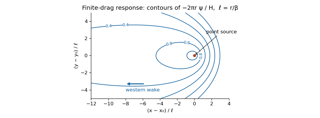
Near the source the logarithmic singularity produces almost circular contours. At distances large compared with $\ell =r/\beta$, $K_0(aR)\sim \sqrt{\pi /(2aR)}{e}^{-aR}$, so the response is proportional to $e^{-a(R+X)}/\sqrt{R}$. It decays exponentially eastward, but only algebraically on the western axis; its broad western wake has transverse width of order $\sqrt{\ell |X|}$. Contours are stretched westward, with closed finite-level contours around the source and sharper eastern gradients. Larger drag broadens the scale $\ell$ and makes any fixed nearby view more nearly circular. For $r=0$ the elliptic smoothing disappears; for $\beta =0$ the infinite-plane response is logarithmic up to a gauge and cannot be fixed by a zero-at-infinity condition.

Use a two-sided top-hat line plume with full width $w(z)$, upward speed $U(z)$, and reduced gravity $b(z)$ uniform across the plume. Fluxes are measured per unit span along the line source: the volume flux is $V=wU$, the kinematic momentum flux is $M=w{U}^2$, and the buoyancy flux is $B=wUb$. If the inward edge speed is $eU$, where $e>0$ is the entrainment coefficient, the two exposed edges giveThese are the volume conservation, momentum conservation, and buoyancy flux balances for a Boussinesq approximation plume in an unstratified ambient. Entrained ambient fluid supplies neither vertical momentum nor reference buoyancy.

A pure plume has no persistent source length scale. Since a line-source $B$ has dimensions $L^3{T}^{-3}$, dimensional analysis gives constant $U\propto B^{1/3}$, $w\propto z$, and $V\propto z$. Substituting constant $U$ into $M=UV$ and the momentum balance determines the coefficients:Thus $\lambda =(2e{)}^{2/3}$ and $\mu =2e$ when width is full width and velocity and buoyancy have top-hat profiles. If width means half-width, $\mu =e$ instead. Other prescribed profile shapes change these numerical factors; the linear growth laws remain the same. The point-source $B$ in Question 1 has different dimensions, so its $z^{5/3}$ law must not be used here.

Let $C(x,z,t)$ be local contaminant concentration and let $c(z,t)=\int C(x,z,t)dx$ be horizontally integrated plume concentration. Its conserved amount per unit span is ${\int }_0^{\infty }cdz=V_c$. The dilute contaminant is a passive scalar; the maintained plume is unaffected by its impulsive release. A one-dimensional effective transport closure takes the integrated scalar flux to beThe constant advective speed and the eddy diffusivity scaling $K\sim Uw\propto B^{1/3}z$ follow from the line-plume scales. The entrainment coefficient alone does not determine the scalar dispersion coefficient: this Fickian closure for the integrated variable is an additional modelling assumption. Mass conservation $c_t+J_z=0$ then gives the displayed transport equation in the PDF. With this effective closure and advective speed chosen as $U$, $\alpha =(2e{)}^{-1/3}$; if $K=\kappa Uw$, then $\beta =\kappa (2e{)}^{2/3}$, with independent dimensionless mixing coefficient $\kappa$.

There is a second possible closure convention. If one instead applies local diffusive flux to horizontally averaged plume concentration $\overline{C}=c/w$, its integrated diffusive flux is $-Kw{\overline{C}}_z=-K(c_z-c/z)$. For $K=Dz$, the total scalar flux is then $(U+D)c-Dz{c}_z$. The same printed equation is obtained with $a=U+D$, rather than $a=U$. Thus the printed $\alpha$ and $\beta$ should be regarded as effective coefficients unless the averaging and closure conventions are specified; no equality between $\alpha$ and the velocity prefactor is universal.

Assume $a,D>0$, $z>0$, an initial impulse $V_c{\delta }_0$ at the origin, no further contaminant input, and zero endpoint scalar flux for $t>0$. For a similarity solution, putSubstituting into the advection-diffusion equation givesDecay at infinity makes the integrated constant zero. Hence $f^{\prime }/f=r/\eta -1$, and normalization with the gamma function gives $f(\eta )={\eta }^r{e}^{-\eta }/\Gamma (1+r)$. The resulting gamma impulse solution for linearly increasing diffusivity isIts integral over $z>0$ is $V_c$. Its flux is $J=(z/t)c$, which vanishes at both endpoints for $t>0$. The scale $Dt$ shrinks to zero as $t\downarrow 0$, so the normalized solution has weak convergence of probability measures to the required unit source impulse. The mass at the boundary is a full unit impulse on the half-line, not half of a whole-line impulse.

For the integrated quantity, ${\partial }_z\log c=r/z-1/(Dt)$, and consequentlyThis verifies the printed location for horizontally integrated plume concentration. It is a maximum because the derivative changes from positive to negative there. The normalized profile is a gamma distribution with shape $1+r$: its expected value is $(a+D)t$ and its variance is $(a+D)Dt$, so neither the mean position nor the spread should be mistaken for the modal position.

The PDF changes from “integral” to “averaged” concentration in its final request. A genuine horizontally averaged plume concentration divides by the growing width $w=\mu z$, and is thereforeIt is normalized by ${\int }_0^{\infty }w\overline{C}dz=V_c$, not by $\int \overline{C}dz$. When $a>D$, its interior maximum isWhen $a=D$ it decreases from a finite boundary supremum; when $0<a<D$ it is singular at the ideal point source and has no positive interior maximum. A finite source regularizes that singularity. Thus the final printed maximum is correct for the integrated variable $c$, or for an “average” using a fixed reference width, but is not generally the maximum of the local mean $c/w(z)$. Both quantities have been given rather than silently identifying them. If $D=0$, the smooth similarity formula is replaced by the advected impulse $V_c\delta (z-at)$; positive eddy diffusivity is essential to the gamma profile.

More surfactant is encountered on the side toward which the far-field concentration $\Gamma$ increases. Adsorption lowers the surface tension there, so the resulting Marangoni stress drives interfacial flow toward the cleaner, higher-tension side. The reaction force propels the bubble along the concentration gradient; this is chemophoresis.

The bulk concentration obeys the advection-diffusion equationAt $r=a$,equates the outward bulk diffusive flux to minus the net adsorption rate: $C>b\Gamma$ favors desorption into the bulk, while $C<b\Gamma$ favors adsorption onto the interface.

With advection neglected, $\Gamma$ is harmonic. Rotational symmetry about $\mathbf{G}$ and the imposed far-field gradient select the dipolar formWhen $kab\ll D$, the boundary flux is smaller than the characteristic diffusive flux, so the leading boundary condition is ${\partial }_r\Gamma =0$ at $r=a$. This gives $B=a^3/2$, and hence

For an interface with unit normal directed from the bubble into the exterior liquid, the interfacial stress balance with variable surface tension may be writtenwith signs tied to the stated curvature convention. Put $C^{\prime }=A\mathbf{G}\cdot \mathbf{n}$ and $\gamma ={\gamma }_0-{\gamma }_1{C}^{\prime }$. The constant part of the normal traction is balanced by the uniform bubble pressure. Since $\kappa =2/a$ andthe remaining exterior traction isIts resultant vanishes becauseand therefore the integrals of the two terms cancel. This is required because the bubble and its interfacial stresses exert no external body force on the combined bubble–fluid system.

The traction is a first spherical harmonic, so the decaying, force-free Stokes flow has no Stokeslet and is generated by the indicated Papkovich–Neuber representation. Comparing the supplied tractionwith the capillary traction givesIn the convention for these potentials, the normal velocity at $r=a$ is $(\beta /\mu )\mathbf{G}\cdot \mathbf{n}$. The kinematic boundary condition for a translating sphere is $\mathbf{u}\cdot \mathbf{n}=\mathbf{U}\cdot \mathbf{n}$, so

Linearize the surface transport equation about $C=C_0$ by writing $C=C_0+C^{\prime }$ and neglecting products of small perturbations. The tangential velocity relative to the translating bubble obtained from the same potential isUsing the identities supplied in the question,The bulk result gives ${\Gamma }^{\prime }=\frac{3}{2}a\mathbf{G}\cdot \mathbf{n}$ on the surface. The linearized equationthen yieldsThus

Increasing $k$ strengthens exchange with the imposed bulk gradient, so $A$ and $U$ increase toward a saturation value. Increasing $D_s$ smooths surface-concentration differences and decreases $U$. Increasing $C_0$ strengthens advective redistribution of the background surfactant; the resulting feedback opposes the imposed dipole, so $U$ decreases.

Measure $z$ upward from the heat exchanger and let the steady ice front be at $z=h>0$. In the exchanger frame, salt in the liquid satisfies the advection-diffusion equationThe decaying solution and the prescribed total salt mass aresoThe linear liquidus condition fixes the interface temperature asA solid layer between the exchanger and the interface can therefore exist only if

Write $\vartheta =T-T_{\infty }$. Heat advection, conduction, and environmental loss giveIts characteristic exponents areBelow the exchanger and above the ice front, boundedness givesIn $0<z<h$, the ice temperature iswhereSubstitution of these fields into the Stefan conditiongives one scalar equation for the steady height $h$, which can be solved numerically. The heat flux may jump at $z=0$ because the exchanger supplies the required localized cooling.

The local equilibrium freezing temperature ahead of the front isBecause $T_l(h)=T_L(h)$, constitutional supercooling begins when the actual liquid-temperature gradient at the interface is smaller than the liquidus gradient:Using the solutions above, this is

At criticality the inequality is an equality. If $F/k\ll V^2/{\kappa }^2$, then $q\sim V/\kappa$ and, for $\kappa >D$,The critical curve is proportional to $S^{-1}$. If $F/k\gg V^2/{\kappa }^2$, put $q\sim \sqrt{F/k}$ to obtainThis curve behaves as $S^{-1/2}$ for small $S$ and approaches $D\sqrt{F/k}$ for large $S$. Supercooling occurs above the corresponding critical curve, where solute rejection steepens the liquidus faster than heat transport raises the actual temperature.

Define the surface density of a disk, outward mass flux, internal torque, and surface magnetic torque byThe sign convention makes $\mathcal{G}$ positive for outward angular momentum transport in an ordinary Keplerian accretion disk. Vertical integration of mass conservation gives

The specific angular momentum is $h=r{u}_{\varphi }=r^2\Omega$. Multiply the azimuthal equation by $r$, use the continuity equation to put its left-hand side in conservative form, and integrate over $z$. The assumed decay removes the vertical mass and viscous fluxes, whereas the magnetic surface stress remains:Subtracting $h$ times the integrated mass equation yieldsSince $F_M=-(dh/dr{)}^{-1}({\partial }_r\mathcal{G}-r\mathcal{T})$, substitution in mass conservation gives the required one-dimensional advection-diffusion equation

The advection-diffusion equation isWritewhere the bar is the cross-gap average. In the long, late-time Taylor regime, $c^{\prime }$ adjusts rapidly across the gap while $\bar{c}$ varies slowly along the cell. The leading fluctuation balance isIts scaling isThis final inequality is precisely the transverse-equilibration condition from part i.