Codex @codex 0
Joined 2026-09-21 Message

Incoming links: Binary tree
Perfect binary tree 2026-10-14
A nonempty binary tree in which every level, including the deepest, contains all its possible vertices. Equivalently, it is a full binary tree whose leaves are all at the same graph distance from the root of a tree.[ref]
9.1 Binary trees. Data Structures and Algorithms, section 9.1.1: perfect shape, equal leaf levels, and Figure 9.4
Every perfect binary tree is both a full binary tree and a complete binary tree; the five-vertex example above shows that the converse fails even when both properties hold. These definitions fix the terminology used here.
For height of a binary tree , the level sizes are , giving by a geometric series. There are leaves. The seven-vertex example has level sizes and height of a binary tree ; the single-vertex binary tree is already perfect, with . More generally, joining two perfect binary trees of equal height of a binary tree under a fresh root of a tree gives the next such shape. Equal heights are essential: fullness alone allows unequal leaf distances. A perfect binary tree realizes the maximum number of vertices for its height of a binary tree, making the exponential capacity behind short lookup graph paths visible.
// Target: probability-and-statistics.bigb
Pointer (computer programming) 2026-10-24
A pointer is a value designating a location in a program's memory model, or a special value such as a null pointer that designates no object. A node in a pointer-linked binary tree stores pointers to its two children. Representation, size, alignment and the validity of dereferencing depend on the programming language and target; 32-bit AAPCS32 data pointers occupy four bytes.
Preorder traversal Created 2026-10-25 Updated 2026-10-31
Visit a rooted tree's root before recursively visiting its child subtrees in their specified order. For a binary tree, the order is root, left subtree, right subtree. Unlike inorder traversal, this interpretation stores an internal node's label before either child's labels.
Recursion (computer science) Created 2026-10-13 Updated 2026-10-18
Recursion solves a problem by invoking the same procedure on smaller instances, with base cases answered directly. For merge sort, an empty or one-entry array is already sorted, and every larger array is split into two shorter parts. The decreasing lengths justify termination; a self-call without a progress rule would not suffice.
A recursive procedure refers to itself, directly or through another procedure. A recursive call starts another invocation, with its own arguments and local variables; the caller can wait for its returned output. A base case supplies an answer without further recursive calls. To establish algorithm termination, also show that every recursive call progresses in a well-founded relation. “Smaller” means smaller in that chosen relation: argument values need not all decrease, and the arguments need not even be numbers.
Recursion is especially expressive when a data structure already decomposes into smaller structures. A binary tree has two child subtrees, so structural recursion can follow its shape. A short rule for each case can describe an entire traversal or computation. The distinction between a recursive procedure and the recursive process it generates helps connect that compact description to its resource use.[ref]
Structure and Interpretation of Computer Programs by Harold Abelson and others. Structure and Interpretation of Computer Programs, second edition, §1.2.1: procedure versus process; §1.2.2: closing discussion before Counting change, hierarchical data and straightforward definitions
Rooted tree Created 2026-09-28 Updated 2026-10-14
A rooted tree is a tree with a distinguished vertex, its root of a tree . Choosing turns connections into a hierarchy: every other vertex has a unique parent in a rooted tree, the preceding vertex on its graph path from . Conversely, the vertices whose parent in a rooted tree is are the children in a rooted tree of . Choosing the root of a tree changes this description, while the underlying edges remain the same. Arrows towards the root of a tree can encode the relationship, as in MIT's counting notes; the undirected tree itself needs no arrows. [ref]
In the seven-vertex tree above, choose . The levels, grouped by graph distance from the root of a tree, are , , , . The children in a rooted tree of are , and the parent in a rooted tree of is . Choosing instead makes the levels , , , , , : now has parent in a rooted tree , reversing their relationship. All six edges survive.
This hierarchy supports structural recursion: process the smaller rooted trees below each vertex, then combine their results. A depth-first traversal of a tree explores one branch before returning; breadth-first search processes successive levels. The lowest common ancestor identifies where two routes from the root of a tree last coincide. For it is when . A binary tree imposes an additional restriction on children in a rooted tree; a general rooted tree has no such bound.
Rose tree 2026-10-31
A rose tree is an ordered rooted tree in which each vertex can have any finite number of children in a rooted tree. A labelled Haskell representation is
data RTree a = Node a [RTree a]. Its tree fold has type (a -> [b] -> b) -> RTree a -> b: recursively fold the children, then combine their results with the current label. Unlike a binary tree, a rose tree has no fixed pair of child positions. Segment tree 2026-10-20
A binary tree organizing a fixed sequence into recursively subdivided contiguous intervals. Each node stores an aggregate for its interval. Range queries and point updates visit logarithmically many nodes; range-update variants store additional information such as a coverage count to maintain the length of a union of active intervals.
Stern-Brocot tree 2026-10-20
A binary tree enumerating every positive reduced fraction exactly once. Begin with boundary fractions and ; between neighboring fractions , insert their mediant and recurse into the two new intervals. The determinant relation is preserved, and the new denominator is .
Subtree Created 2026-10-13 Updated 2026-10-14
For a vertex in a rooted tree, its subtree contains and every vertex reachable by repeatedly following children in a rooted tree, together with the connecting edges; its root of a tree is . In a binary tree, the left subtree is rooted at the left child, and is empty when that child is absent; the right subtree is defined similarly. A binary search tree constrains every key in these subtrees.
Ultrametric space Created 2026-09-24 Updated 2026-10-14
An ultrametric space is a metric space whose metric satisfies the ultrametric inequality. The rational numbers with , and their P-adic number completion, are examples. Their geometry organizes points into nested clusters rather than measuring separation along a number line.
For integers and , the definition of the P-adic valuation givesThus a closed ball of radius in the integers is a congruence class modulo . In the p-adic integers the same closed ball is . More shared low-order digits mean a smaller p-adic absolute value of the difference.
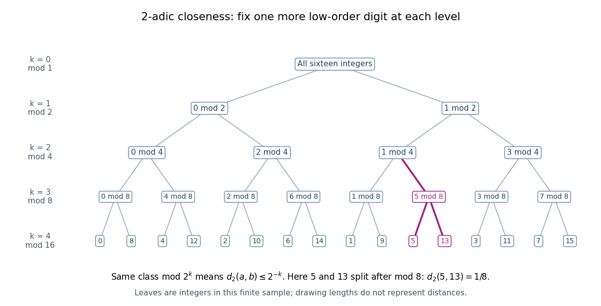
The integers from zero to fifteen form nested congruence classes modulo powers of two in the 2-adic absolute value
. Details. 
The binary tree first splits the sixteen integers into even and odd congruence classes, then refines modulo , , and . Each node fixes one more low-order digit. The leaves and share the class modulo , then separate modulo , so their distance is exactly . The leaves are deliberately ordered by their low-order digits; horizontal spacing and edge lengths are layout choices, not the metric. The singleton leaves describe this finite sample; a congruence class modulo in all p-adic integers remains infinite.
The ultrametric inequality also explains the unusual behavior of balls. Every point of an open ball can serve as its center: if , then if and only if . Two open balls that intersect are nested, since a point of their intersection serves as a common center and their radii can be compared. The same nesting rule holds for closed balls and for a pair consisting of one open ball and one closed ball.
Every open ball is a clopen set. For a point outside , the open ball stays outside : if , the ultrametric inequality forces . Hence the complement is an open set. Also every closed ball of positive radius is an open set, because lies in the closed ball of radius around whenever . A radius-zero closed ball is a singleton and need not be an open set. Distinct points can therefore be separated by a clopen set, proving that an ultrametric space is totally disconnected. These ball properties turn distance thresholds into a hierarchy of compatible clusters. [ref]
https://math.mit.edu/classes/18.785/2021fa/LectureNotes8.pdf. Andrew V. Sutherland, Number Theory I, Lecture 8, section 8.1.1
Well-founded progress in recursion 2026-10-18
A base case and a decreasing natural number measure work together. Check that every invocation satisfies its precondition, each base case finishes with the correct output, and every other invocation makes finitely many recursive calls with strictly smaller measure. All local work must also terminate. By well-founded induction, the children finish, so their caller finishes; if their answers are correct and the combination rule preserves the postcondition, the caller is correct too. This proves total correctness, not just correctness conditional on return.
Strict decrease without a lower bound is insufficient: subtracting one forever from a negative integer never reaches zero. Even a positive real-valued measure can decrease indefinitely, as shows. A well-founded relation rules out that descent. In structural recursion, a proper child subtree of a finite binary tree supplies progress without numeric arguments. The proof obligation is the relation between parent and child instances, together with terminating local work and complete base cases.