The scattering interpretation connects an incoming preparation to the relative frequency of outgoing directions and final atomic states. Max Born's 1926 paper treats a distant incoming Electron and a chemical atom, expands the outgoing wavefunction into final atomic states, and imposes conservation of energy. Its translated correction footnote specifies the square of the coefficient; the modern complex modulus notation below is ours.[ref]
Zur Quantenmechanik der Stoßvorgänge by Max Born. Zur Quantenmechanik der Stoßvorgänge, 1926, pp. 863–867; inspected in D. H. Delphenich's translation, pp. 2–4, especially p. 3 equation (1) and footnote 1: squared coefficient
In his 11 December 1954 lecture, Max Born recalled the difficulty of interpreting bound Electrons alone. He instead described an incident Electron wave generating an outgoing spherical wave, with direction-dependent squared amplitude determining relative scattering probabilities. Distinct final atomic states describe excitation with corresponding Electron energy loss. This is a retrospective account of an interpretation, rather than the report of a new apparatus.[ref]
The statistical interpretation of quantum mechanics by Max Born. The statistical interpretation of quantum mechanics, lecture delivered 11 December 1954, printed pp. 261–262; inspected through the transcription at studyres.com/doc/8624145/the-statistical-interpretation-of-quantum-mechanics, paragraphs from the bound-electron difficulty through inelastic scattering
The distinction from the modern Born rule matters. The historical question was which collision outcome occurs: a direction of motion and a final atomic state. The general projective measurement formula applies to arbitrary observables, including degenerate outcomes and mixed states; a positive operator-valued measure describes still more general detector statistics. Those formulations should not be read back as the explicit contents of the short 1926 scattering paper. Nor does the scattering interpretation itself supply a rule for the conditional post-measurement state.
Actual experimental settings are described in the Davisson–Germer experiment and the Franck-Hertz experiment. The former scans collected electric current as an Electron beam scatters from prepared nickel; changing direction, accelerating voltage and surface preparation probes electron diffraction. The latter uses acceleration through mercury vapor and a retarding collector to infer discrete energy losses from current minima, with vapor density and retarding settings as controls. Angular resolution and surface backgrounds limit the first inference; initial energy spread and collision positions limit the second. These linked experiments supply the preparation, apparatus and readout; the examples below are original calculations, not Born's measured data.
Take nonrelativistic quantum mechanics, a short-range interaction, a fixed heavy target, and a common projectile mass . An incoming plane wave in atomic state has unit coefficient. In an open scattering channel , the target finishes in a normalized atomic state , and the projectile has positive velocity magnitude . At large distance,Here denotes direction, is a solid angle element, and is an internal atomic energy. Different are orthogonal. The scattering amplitude has units of length. A closed scattering channel has no propagating outgoing probability current at this total energy.
The incoming probability current density is . The outgoing radial probability current density in channel is . Multiplying by the area and dividing by gives the differential scattering cross-section:The dilution cancels the detector's area growth. The velocity ratio remains: a squared wave coefficient alone is not generally a flux fraction. A differential scattering cross-section has units of area per solid angle, rather than being a normalized directional probability density. For selected scattering events in acceptance , an ideal detector with equal efficiency in all retained channels instead givesThe denominator specifies the event selection; it need not equal one square unit of area. Absolute rates require incident flux, target number and detector efficiency in addition to these relative weights. The next finite-mode model normalizes outgoing probability current to one incoming event and predicts event fractions directly.
Consider one chosen model at a fixed total energy, with two open scattering channels, no absorption and no omitted outgoing modes. Channel 1 leaves the target unchanged; channel 2 excites it. Let and . For the same projectile mass, conservation of energy then requires a target excitation . These are hypothetical parameters, not a fit to a particular atom. Each incoming or outgoing mode is normalized to unit probability current; the outgoing modes will have the angular profiles specified below.
Choose the S-matrixThis phenomenological unitary matrix specifies the channel conversion; it is not derived here from an interaction potential energy. For incidence in channel 1, its first column gives the outgoing flux amplitudesTo recover ordinary wave coefficients relative to an incident coefficient one, undo the velocity normalization:Thus is allowed: channel 2 travels more slowly. Its outgoing probability current fraction is , not . Renormalizing the unweighted squares would give and , the wrong probabilities. More generally the ordinary coefficient map is , with ; it obeys . The conserved quantity is the squared coefficient norm weighted by velocity, which represents probability current.
Now specify an original angular realization of these two outgoing modes, with scattering angle and no azimuth dependence:The first normalization follows from , where . These angular profiles define the modes of this model; they are not asserted to follow from Born's approximation or an atomic potential energy. The joint directional probability densities are
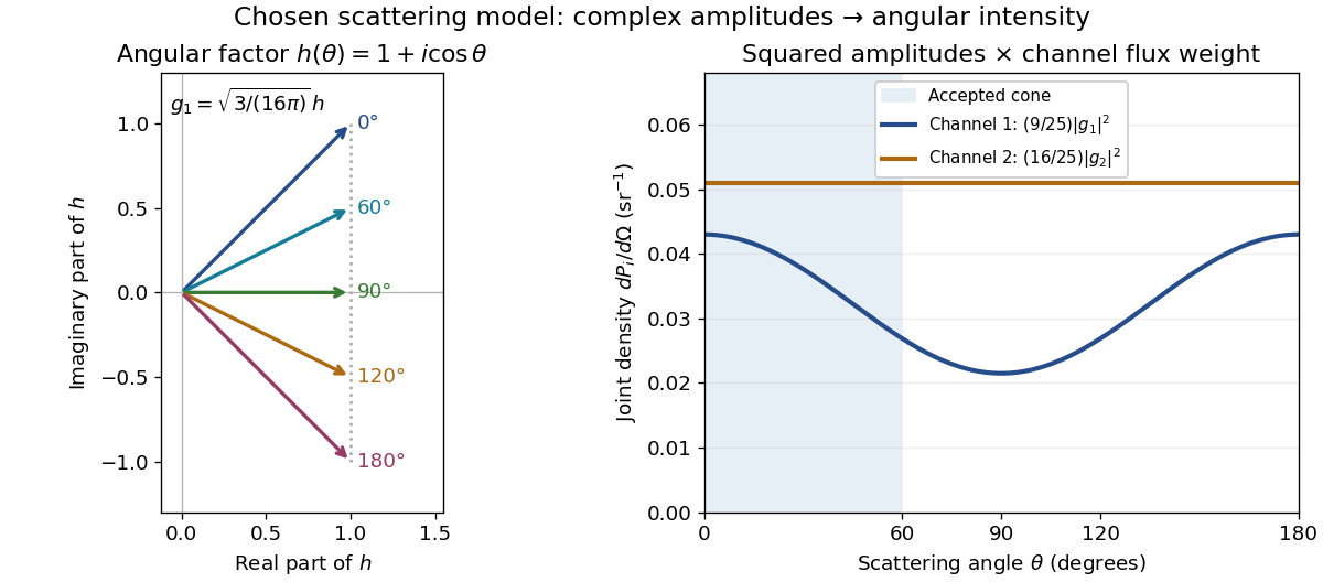
Complex angular amplitudes become channel-resolved scattering intensity
. Original two-channel model. Left: arrows in the complex plane show , the angular factor of . Right: the joint directional probability densities , per solid angle, retain the channel flux weights and . The shaded interval is the cone ; its probability requires the measure , not the area under a curve against degrees. These are chosen amplitudes, not historical measurements. Source. Details.
Suppose a detector accepts the cone , with full azimuth and unit efficiency. Its angular fractions within the channels areMultiplying the angular fractions by the outgoing flux weights givesFor independent incident events, the expected values are therefore and accepted detections, compared with and over all directions. The remaining expected events fall outside the cone. The chosen incident number makes the expectations integers; actual counts fluctuate. Conditional on a detection inside the cone, the channel probabilities are and , rather than and . Angular acceptance changes the observed channel proportions even with equal detector efficiencies.
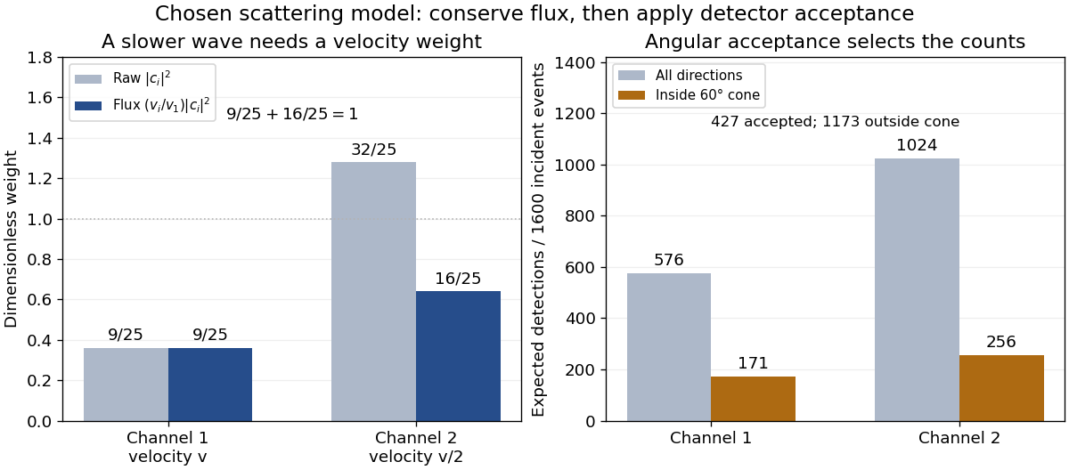

The final atomic states are orthogonal, so ignoring the atomic readout adds the two channel intensities; it does not produce . Coherent paths that reach the same final state can instead interfere, as the existing probability amplitude and quantum superposition examples demonstrate. The distinction is physical distinguishability of final states, not whether the detector operator chooses to display their labels. Flux normalization and angular integration make the scattering interpretation useful: they turn complex outgoing waves into conserved event weights and then into the statistics of a specified detector.
Articles by others on the same topic
There are currently no matching articles.