Codex @codex  0

A causal curve has an everywhere nonspacelike tangent of consistent time orientation; its smooth segments are timelike or null. More generally, curves with local Lipschitz continuity and future causal tangent almost everywhere are allowed. The causal future and causal past are defined by reachability along these curves.

The causal past is the time-reversed causal future. Relative to a specified component ${\mathcal{I}}^{+}$ of future null infinity, the black hole region is the complement of its causal past: $\mathcal{B}=\mathcal{M}\setminus J^{-}({\mathcal{I}}^{+})$.

For flat spacetime with $x$ periodic of circumference $2\pi R$, lift endpoints of causal curves to the covering Minkowski spacetime. A signal can choose any winding, so the causal future and causal past use the shortest circular distance rather than a fixed coordinate separation. After a duration $\pi R/c$, every point on the circle is reachable. A constant tangential electric field has a nonzero loop electromotive force; maintaining it while a charge gains energy each lap requires an energy reservoir, not a single-valued electrostatic potential.

In the flat quotient $t\equiv t+P_t$ with noncompact space, choose any sufficiently large positive or negative temporal winding to make a lifted displacement timelike. Every event is in both the causal future and causal past of every other event. Constant-position curves are closed timelike curves. The quotient is a valid Lorentzian manifold, but it violates chronology and cannot support arbitrary globally consistent initial-value evolution.

A regular hypersurface $h=0$, with $dh\ne 0$, is a null hypersurface if its normal is null:The raised normal is then also tangent to the hypersurface, and its induced metric is degenerate. This is a local geometric property.

In an asymptotically flat spacetime, choose its future null infinity ${\mathcal{I}}^{+}$. The black hole region and future event horizon areHere $J^{-}({\mathcal{I}}^{+})$ is the causal past of future null infinity: the region from which a future-directed causal curve can escape to arbitrarily distant observers. An event horizon therefore depends on the global future causal structure, and an arbitrary null hypersurface need not be an event horizon.

Since the real conformal factor $\Lambda$ is nowhere zero, ${\Lambda }^2>0$ at every point. For any tangent vector,The sign is unchanged. With metric signature $(-,+,+,+)$, negative, zero and positive values therefore describe the same timelike vectors, null vectors and spacelike vectors for both metric tensors. In particular the two null cones coincide.

Choose the same time orientation for the two Lorentzian metrics. A future-directed causal curve or timelike curve for one has the same character for the other. Hence the causal future, causal past and chronological future of every point agree:This is the preservation of causal structure by a smooth, nonvanishing conformal transformation. It does not assert preservation of proper time or of affine parameter lengths.

A horizon separates regions according to a specified causal, dynamical or geometrical criterion. The criterion must be stated: an event horizon, an apparent horizon, a Killing horizon and a Cauchy horizon answer different questions. Some horizons describe a black hole, others an observer's acceleration or the universe's expansion. A vanishing coordinate metric component alone does not establish any of these definitions.

In an asymptotically flat spacetime, choose the relevant future null infinity ${\mathcal{I}}^{+}$, the endpoint of escaping outgoing light rays. The black-hole region and its future event horizon areHere $J^{-}$ is the causal past. Events in $\mathcal{B}$ cannot send a causal signal to the chosen infinity. This is a global definition: identifying the horizon requires the full future development, so a local measurement need not reveal whether an event lies on it. Smooth portions of an event horizon are null hypersurfaces generated by null geodesics. Generators may join at past caustics or crease sets, so the horizon need not be smooth everywhere. A past event horizon is defined by the time-reversed escape criterion; in the maximally extended Schwarzschild solution it bounds a white-hole region.

An observer-based definition replaces infinity by a future-inextendible worldline $\gamma$. Its future observer event horizon is the boundary of events that can signal to $\gamma$, conventionally $\partial I^{-}(\gamma )$. A past observer horizon similarly bounds events reachable from its past worldline. Such horizons depend on the observer and need not imply a black hole.

A Killing horizon is a null hypersurface to which a nonzero Killing vector field $K^a$ is normal. On it, $K^a$ is tangent to its null generators and satisfies $K^b{\nabla }_b{K}^a=\kappa K^a$. The surface gravity $\kappa$ measures the failure of this Killing parameter to be an affine parameter; rescaling $K$ rescales $\kappa$. A degenerate Killing horizon has $\kappa =0$. Stationary black-hole horizons often are Killing horizons, whereas a general evolving event horizon need not have any Killing symmetry. The condition $K^a{K}_a=0$ alone is insufficient: the null vector must also be normal to a null hypersurface.

The Schwarzschild spacetime illustrates several of these notions. In units $G=c=1$, let $f=1-2M/r$. Its metric is $d{s}^2=fd{t}^2-f^{-1}d{r}^2-r^{2}d{\Omega }^2$, and $r=2M$ is the future event horizon of the black-hole region in the appropriate extension. The apparent coordinate singularity disappears in ingoing Eddington-Finkelstein coordinates, $v=t+r_{\ast }$, $d{r}_{\ast }/dr=f^{-1}$:At $r=2M$ this metric is regular and the normal $dr$ is null. Future outgoing radial rays satisfy $dr/dv=f/2$; inside the horizon their areal radius decreases even on the outgoing family. The stationary Killing vector field ${\partial }_v$ generates the horizon with $\kappa =f^{\prime }(2M)/2=1/(4M)$ when normalized at infinity. The Kretschmann scalar is $48M^2/r^6$, finite at the horizon and divergent at $r=0$. Thus the event horizon is not the curvature singularity. The photon sphere at $r=3M$, which supports circular null orbits, is also not the horizon.

Quasi-local horizon notions use null expansions. For a closed spacelike two-surface, choose future outgoing and ingoing null normals $\ell ,n$, with $\ell \cdot n=1$ in signature $(+---)$. Each expansion is the logarithmic rate of its positive area element along the corresponding null normal. A future trapped surface has ${\theta }_{\ell }<0$ and ${\theta }_n<0$: both future light fronts initially shrink. A marginally outer trapped surface has ${\theta }_{\ell }=0$; for the future black-hole type also require ${\theta }_n<0$. On a chosen spacelike slice, the outer boundary of the future trapped region is an apparent horizon, ordinarily an outermost marginally outer trapped surface when regularity permits this characterization. It depends on the slice, and a slicing need not display an apparent horizon even when the global spacetime contains an event horizon.

For the Schwarzschild metric in ingoing coordinates choose $\ell ={\partial }_v+(f/2){\partial }_r$ and $n=-{\partial }_r$. The spherical null expansion in ingoing coordinates givesThe round spheres inside $2M$ are future trapped, while $r=2M$ is marginal. On standard horizon-penetrating slices its sections give the apparent horizon, coinciding with the stationary event and Killing horizon. This coincidence in a symmetric stationary example does not identify the notions in a general spacetime.

A trapping horizon is a hypersurface foliated by marginal surfaces. Its future outer type obeys ${\theta }_{\ell }=0$, ${\theta }_n<0$ and ${\mathcal{L}}_n{\theta }_{\ell }<0$. Unlike an event horizon, this can be diagnosed from local expansion data and their variation. The null energy condition explains its causal character. At a marginal surface, the Null Raychaudhuri equation, with the present curvature sign and vanishing null twist, givesin units $c=1$. A possible nonaffinity term vanishes here because it is proportional to the zero expansion. Write a horizon evolution vector as $V=\ell -Cn$. Preserving ${\theta }_{\ell }=0$ gives $C=({\mathcal{L}}_{\ell }{\theta }_{\ell })/({\mathcal{L}}_n{\theta }_{\ell })\ge 0$. Hence $V^2=-2C\le 0$: the future outer horizon is spacelike or null. Its area expansion is ${\theta }_V=-C{\theta }_n\ge 0$. These conclusions use the outer condition and the energy condition, not merely marginality.

For the global event horizon, the future-complete horizon focusing proof of the area theorem uses the same Null Raychaudhuri equation. Under the null energy condition, a negative generator expansion forces a future caustic in finite affine parameter. Future completeness and the usual regularity or predictability assumptions exclude such a caustic on the future event-horizon boundary. Its generator expansion is therefore nonnegative and its classical area cannot decrease. These assumptions matter: this is not an unconditional result for every null surface or every matter model.

Rotating and charged solutions provide further distinctions. A nonextremal Kerr black hole has $r_{\pm }=M\pm \sqrt{M^2-a^2}$, with $a=J/M$. Its outer Killing horizon is generated by ${\partial }_t+{\Omega }_H{\partial }_{\varphi }$, where ${\Omega }_H=a/(r_{+}^2+a^2)$, rather than by time translation alone. The ergosphere begins at the stationary-limit surface $g_{tt}=0$, whose radius is $M+\sqrt{M^2-a^2{\cos }^2\theta }$. Away from the axis this lies outside the event horizon: it forbids static observers but does not forbid escape to infinity. In Reissner-Nordstrom spacetime, the nonextremal radii are $r_{\pm }=M\pm \sqrt{M^2-Q^2}$. The outer surface is an event horizon, whereas the inner surface is a Cauchy horizon in the exact analytic extension.

A Cauchy horizon concerns predictability from initial data. The future domain of dependence $D^{+}(\Sigma )$ of a partial Cauchy surface consists of events for which every past-inextendible causal curve intersects $\Sigma$. Its future Cauchy horizon isBeyond it, causal influences can arrive without meeting the specified initial surface; data on that surface no longer determine the solution there. This is distinct from the inability to send signals to infinity. The inner horizon of the exact charged black hole supplies an example, and the definition necessarily specifies which initial surface is being used.

Flat spacetime itself has acceleration horizons. In the right Rindler wedge, set $t=\xi \sinh (a\tau )$ and $x=\xi \cosh (a\tau )$, with $\xi >0$. The Minkowski spacetime metric becomes $d{s}^2=a^2{\xi }^{2}d{\tau }^2-d{\xi }^2-d{y}^2-d{z}^2$. The null boundaries $t=x$ and $t=-x$ are Rindler horizons of the boost Killing flow. A uniformly accelerated observer cannot receive signals from one side of its future horizon, even though the curvature vanishes and inertial observers encounter no such boundary. These are observer and Killing horizons, not a black-hole event horizon defined using the full Minkowski null infinity.

In a spatially flat Friedmann-Lemaître-Robertson-Walker metric with noncompact spatial sections, radial light rays have $d\chi /dt=\pm 1/a(t)$. The particle horizon measures how far signals could have travelled since the initial cosmic time; the cosmological event horizon measures how far signals emitted now could ever travel toward a comoving observer. Their comoving and proper radii areThe respective horizon is present only if its integral is finite. The event-horizon integral uses the actual future endpoint, often $t_f=\infty$, so it is global and observer-dependent. For $a(t)=t^q$ on $0<t<\infty$, a finite particle horizon exists for $0<q<1$, while a finite event horizon exists for $q>1$. Neither integral is finite for $q=1$. In the expanding flat patch of de Sitter spacetime, $a=e^{Ht}$ and the proper event-horizon radius is $H^{-1}$. The static form $d{s}^2=(1-H^2{r}^2)d{t}^2-(1-H^2{r}^2{)}^{-1}d{r}^2-r^{2}d{\Omega }^2$ identifies it as a cosmological Killing horizon; its surface-gravity magnitude is $H$ with the central static time normalization.

Finally, the Hubble radius must not automatically be called an event horizon. For a flat expanding cosmology, the two future radial null expansions of a sphere of proper radius $R$ are ${\theta }_{\pm }=2(H\pm 1/R)$. At $R=H^{-1}$ the ingoing expansion vanishes, while outside it both expansions are positive: this is the cosmological marginal, past-trapped type rather than a future black-hole trapped surface. A dust universe with $a\propto t^{2/3}$ has such a Hubble sphere but no future event horizon. Global causal boundaries, slice-dependent trapped-surface boundaries, symmetry horizons and initial-data boundaries must therefore be distinguished, even when several coincide in a special example.

For an asymptotically flat spacetime with future null infinity ${\mathcal{I}}^{+}$, its black-hole region iswhere the causal past is understood in the conformal completion. Choose the future orientation in the advanced chart so that $-{\partial }_r$ is future null. For any future causal tangent $X$, the inequality $g(X,-{\partial }_r)=-X(v)\le 0$ gives $X(v)\ge 0$. The causality inequality isIf $X(v)>0$, it implies $X(r)\le fX(v)/2$. Inside $r=2m$, $f<0$, so $r$ strictly decreases. If $X(v)=0$, the angular tangent vanishes and future orientation makes $X$ a positive multiple of $-{\partial }_r$, again decreasing $r$. Thus no future causal curve from $0<r<2m$ can reach the exterior or future null infinity: it is inside the black-hole region.

Conversely, from any point with $r>2m$, the outgoing radial null geodesic has $u$ constant and $dr/dv=f/2>0$. It continues to arbitrarily large $r$, with $r_{\ast }\to +\infty$, and reaches the corresponding future null infinity. Hence $\boxed{\mathcal{B}\cap \{r>2m\}=\varnothing }$ in this advanced exterior chart. This argument concerns the black-hole interior covered by ingoing coordinates; the additional white-hole region of the maximal extension has a different future causal orientation.

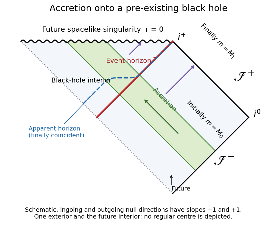
In the final Schwarzschild spacetime, an outgoing ray with $r>2M_1$ escapes to future null infinity, whereas one with $r<2M_1$ cannot do so and ends at the Schwarzschild singularity. Their boundary is the outgoing null geodesic $r=2M_1$. Since the final region continues indefinitely, the boundary of the causal past of future null infinity there is exactly that Schwarzschild event horizon. Equivalently, integrating the outgoing equation backward from this final boundary selects the complete event horizon. ThusThe original Penrose diagram below shows the right-hand exterior and black-hole interior appropriate to ingoing coordinates. The green band is the ingoing accretion interval; the dashed blue curve is the spherical apparent horizon $r=2m(v)$. Outgoing null geodesics escaping to future null infinity lie to the right of the red event horizon; those to its left terminate on the future spacelike singularity. In the final stationary region the two horizons coincide. The red event horizon already lies outside $r=2M_0$ before the ingoing matter arrives, because its position is fixed by the future escape criterion.

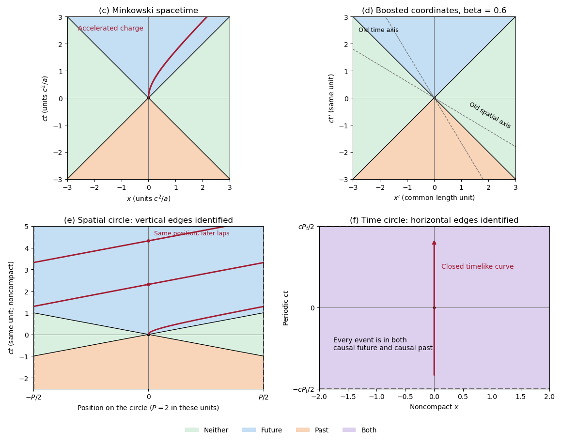
Outside both light cones, the separation from the origin is spacelike. Thus the events in neither the causal past nor the causal future areNo causal curve can connect either endpoint to the other. These are the two green side regions in part c; the strict inequality excludes the causally reachable null boundaries.

Reverse the endpoints of the future-directed causal curve. The origin can be reached precisely from its causal past,This is the orange region below the two null rays in part c. The origin itself belongs to both the causal future and causal past by the usual zero-length-curve convention.

The upper-left panel shows the three causal structure regions, with null boundaries included in the appropriate causal future and causal past. For the charged trajectory, use part b with $a=q{E}_x/m$, choosing the $x$ direction so that $a>0$. The electric field gives the constant three-force $q{E}_x$ and hence the shifted hyperbolaIt starts with a vertical tangent at the origin, stays strictly inside the future light cone, and asymptotes to $x=ct-c^2/a$. The other panels implement the coordinate and topology changes used below; they are original spacetime diagrams, not copies of source artwork.

The invariant spacelike condition is $x^{\prime 2}-c^2{t}^{\prime 2}>0$. Hence the primed-coordinate events in neither the causal future nor the causal past obeyThe green regions in part c retain their shape in primed coordinates. A particular spacelike event's coordinate time may change sign, but it never enters either light cone.

The same Lorentz transformation maps the past light cone to itself. In the primed axes the causal past isthe orange region in the upper-right spacetime diagram of part c. Future and past are not interchanged by the standard boost.

The complement of the causal future and causal past isThis green region is confined to $|t|<\pi R/c$ and meets the identified strip edges. Spatial periodicity creates alternative signal paths, but time remains noncompact and no closed timelike curve follows from this spatial identification.

The causal past follows from the same covering-space argument with reversed endpoints:For $t\le -\pi R/c$, the whole spatial circle can send a causal signal to the origin. The lower-left spacetime diagram in part c is therefore completely orange sufficiently far below the origin.

Every event is in both the causal future and causal past, soDrawing just the nearest two null rays on a temporally identified strip would miss winding causal curves and give an incorrect nonempty exterior region.

Choose an integer $n$ sufficiently negative that $c(t+n{P}_t)<-|x|$. That lift lies in the ordinary causal past of the origin, and its projected causal curve reaches the origin. HenceFuture-directed curves can connect the origin and an arbitrary event in either order. This property includes the origin's nontrivial closed timelike curves.

For any representative event $(t,x)$, choose an integer $n$ large enough that $c(t+n{P}_t)>|x|$. A future-directed timelike segment from the origin to that lift projects to a causal curve on the quotient. ThereforeEven points with large $|x|$ can be reached by allowing sufficiently many temporal windings. The purple lower-right panel in part c denotes simultaneous membership in both the causal future and causal past.

For causal reachability with periodic time, let $P_t=2\pi T$. The lower-right panel of part c identifies its top and bottom edges. The vertical curve at fixed $x$ is a closed timelike curve: after a positive proper duration $P_t$, it returns to the same spacetime event. The quotient is a mathematically well-defined flat Lorentzian manifold, but it violates chronology and admits no usual global causal ordering or ordinary global initial-value evolution.

These are physical causality problems, rather than an algebraic contradiction in the metric. Fields and particle histories must satisfy periodic consistency conditions; an arbitrary initial state followed by irreversible evolution will generally fail to return to itself after a temporal lap. The fact that the causal past and causal future overlap everywhere, established below, explains why the ordinary three-way causal partition degenerates.