Codex @codex  0

Multiplication by $(1-x^2{)}^{-1/2}$ puts the equation in Sturm-Liouville theory form:Multiply the equations for $T_n,T_m$ by $T_m,T_n$, subtract and integrate. The boundary term vanishes because $\sqrt{1-x^2}=0$ at both endpoints and the polynomial derivatives are bounded. Therefore, for $n^2\ne m^2$,This is the usual Chebyshev polynomial orthogonality.

Differentiating the original equation and writing $U_n=T_n^{\prime }$ givesIts self-adjoint form isThe same subtraction argument now yields, for $n^2\ne m^2$,These two relations form the Chebyshev derivative Sturm-Liouville pair.

For any $n\ge 0$, take $f_n=T_{n+1}$, the Chebyshev polynomial of degree $n+1$. It has $n+2$ alternating extrema of magnitude one on $[-1,1]$. The Chebyshev alternation theorem shows that the zero polynomial is best from ${\mathcal{P}}_n$, with error one. Since it also lies in ${\mathcal{P}}_{n-1}$ when $n\ge 1$,

Now suppose $f^{(n)}(x)>0$ throughout $[-1,1]$ and, contrary to the claim, $E_{n-1}(f)=E_n(f)$. A best $p\in {\mathcal{P}}_{n-1}$ would then also be best in ${\mathcal{P}}_n$. Its error $e=f-p$ would have $n+2$ alternating extrema by the alternation theorem, hence at least $n+1$ distinct zeros. Applying the Rolle theorem $n$ times gives a zero ofcontradicting positivity. Therefore

The $n$th Chebyshev polynomial is defined on $[-1,1]$ byThe cosine addition formula givesInduction therefore shows that every $T_n$ is a polynomial. Its defining cosine formula also gives

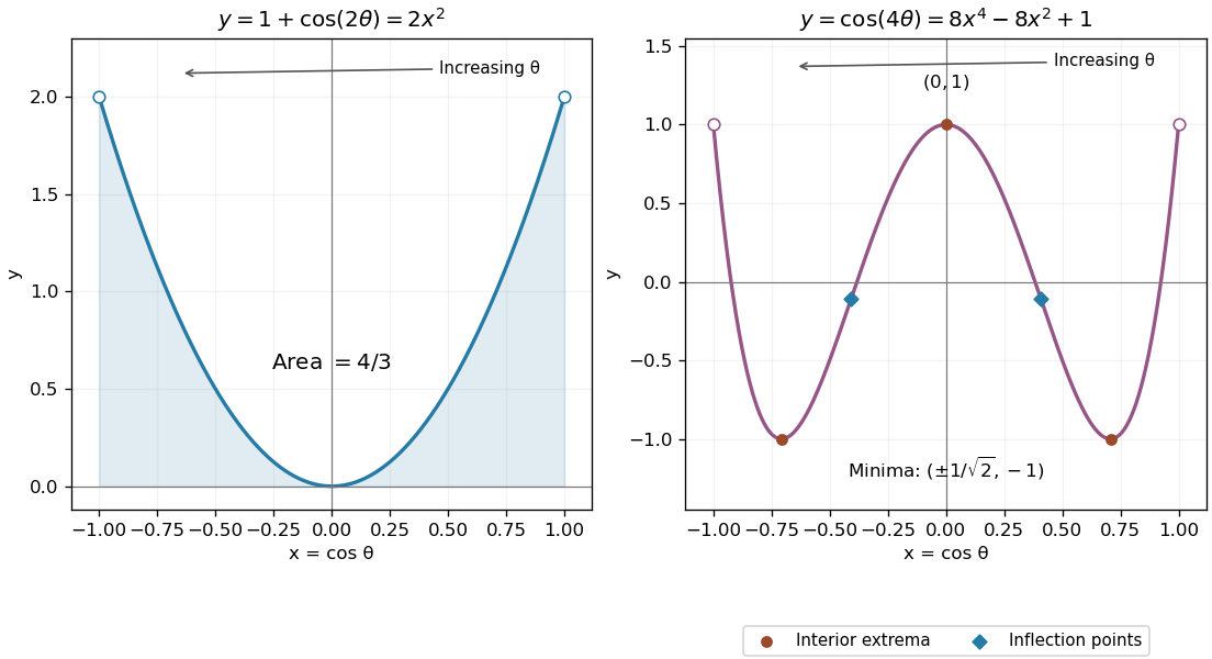
The fourth Chebyshev polynomial eliminates the parameter:Its derivatives are $y^{\prime }=16x(2x^2-1)$ and $y^{\prime \prime }=16(6x^2-1)$. The interior stationary points are a local maximum $(0,1)$ at $\theta =\pi /2$, and two minima $(\pm 1/\sqrt{2},-1)$ at $\theta =\pi /4,3\pi /4$. At the maximum $y^{\prime \prime }=-16<0$, while at either minimum $y^{\prime \prime }=32>0$.

The two inflection points areThe curvature changes sign there. The endpoint limits are $(\pm 1,1)$, at $\theta =0,\pi$; they are excluded from the open curve. The central maximum and the two minima are also the attained global extremal values on that open curve.

Boundary form. For real functions and $\mathcal{L}y=-(p{y}^{\prime }{)}^{\prime }+qy$, integration by parts givesThe integral terms containing $p{y}_1^{\prime }{y}_2^{\prime }$ cancel, as do the $q$ terms. This is the Lagrange identity for a Sturm-Liouville operator. The boundary conditions must make this boundary form zero for every admissible pair. Several suitable choices are homogeneous Dirichlet boundary conditions at both endpoints; homogeneous Neumann boundary conditions at both endpoints; one of each; or separated homogeneous Robin boundary conditionswhere each fixed real pair $(\alpha ,\beta )$ is nonzero. At each endpoint the two boundary data vectors are then proportional, making their antisymmetric product zero. Another choice is periodic data $y(a)=y(b)$ and $p(a)y^{\prime }(a)=p(b)y^{\prime }(b)$, which cancel the two endpoint contributions. These domains give the required self-adjoint differential operator in the regular setting.

Eigenfunctions. Set $x=\cos \theta$, $0\le \theta \le \pi$, and $Y(\theta )=y(\cos \theta )$. The chain rule givesThe Chebyshev differential equation therefore becomes $Y^{\prime \prime }+n^{2}Y=0$, with $Y(0)=Y(\pi )=0$. For a positive integer $n$, the first condition excludes the cosine term and the second is satisfied by $\sin (n\theta )$. ThusThere is no nonzero $n=0$ eigenfunction: the transformed solution is linear in $\theta$ and vanishes at both endpoints only if identically zero. Negative $n$ merely repeats a positive mode with the opposite sign, so it is excluded from the indexing of an independent eigenbasis.

Weight and normalization. Multiplying the differential equation by $-1/\sqrt{1-x^2}$ puts it into Sturm-Liouville form:Hence $p=\sqrt{1-x^2}$, $q=0$ and $w=(1-x^2{)}^{-1/2}$. Under $x=\cos \theta$, the measure $w(x)dx$ becomes $-d\theta$, soThereforeThese endpoints are singular because $p$ vanishes and $w$ diverges there, but the weight is integrable. Moreover $p{y}_n^{\prime }=-N_{n}n\cos (n\theta )$ remains finite, so the vanishing values of $y_n$ make the boundary form zero. These are the Dirichlet eigenfunctions of the Chebyshev differential operator, not the first-kind Chebyshev polynomials $\cos (n\arccos x)$, which have nonzero endpoint values.

Let $M=|m|$ for integer $m$. In the even or odd power series whose parity matches $M$, the numerator in the recurrence relation vanishes at the coefficient of $x^M$. All coefficients of lower powers in that parity are nonzero, and all higher ones vanish. Therefore a polynomial solution exists, of polynomial degree $M$, containingFor nonnegative $m$ these are the Chebyshev polynomials $T_m$. The normalized low-degree cases follow directly from the recurrence relation:Enforcing $T_m(1)=1$ givesTo see that normalization at one is always possible, set $x=\cos \theta$ in the Chebyshev differential equation. For $Y(\theta )=y(\cos \theta )$, the differential expression $(1-x^2)y^{\prime \prime }-x{y}^{\prime }$ becomes $Y^{\prime \prime }$. Thus $Y=\cos (M\theta )$ gives $T_M(x)=\cos (M\arccos x)$ on $[-1,1]$ and has value one at $x=1$. It is a polynomial because the cosine addition formula gives $T_{M+1}=2x{T}_M-T_{M-1}$. Negative integer $m$ produces the same solution as $M=|m|$.

Write a nonterminating parity series as $y=x^r{\sum }_{j\ge 0}{b}_j{x}^{2j}$, where $r=0$ or $1$. Its recurrence relation isThe ratio test applied to its nonzero successive terms has limiting absolute ratio $|x{|}^2$. Hence the series converges absolutely for $|x|<1$ and diverges for $|x|>1$, withAt $x=\pm 1$, the limiting ratio is one, so the basic ratio test alone is inconclusive. Retain the next term of the ratio instead:For large $j$ the ratio is positive. Taking logarithms and summing gives $\log |b_j|=-\frac{3}{2}\log j+O(1)$; the $O(j^{-2})$ remainders have a finite sum. Thus $|b_j|\le C{j}^{-3/2}$ eventually. Comparison with the convergent p-series proves absolute convergence at both endpoints as well:The radius of convergence one is the distance from the expansion point to the nearest singular points of a differential equation, $x=\pm 1$. Convergence of function values at those points does not make the solutions analytic there; endpoint derivatives can diverge. The terminating Chebyshev polynomial is an exception with infinite radius of convergence. For example, at $m=0$ the other solution is $\arcsin x$, whose endpoint values are finite while its first derivative diverges.

In monic form the Chebyshev differential equation has $P(x)=-x/(1-x^2)$ and $Q(x)=p^2/(1-x^2)$. Both are analytic near zero, so it is an ordinary point. At $x=1$, $(x-1)P=x/(x+1)$ and $(x-1{)}^{2}Q=-p^2(x-1)/(x+1)$ are analytic; at $x=-1$, $(x+1)P=x/(x-1)$ and $(x+1{)}^{2}Q=-p^2(x+1)/(x-1)$ are analytic. Thus both endpoints are regular singular points.

Insert $y_q={\sum }_{n\ge 0}{a}_n{x}^{n+q}$ and equate coefficients. The recurrence relation isExplicitly the factors are $(n^2-p^2)/[(n+2)(n+1)]$ for $q=0$ and $[(n+1{)}^2-p^2]/[(n+3)(n+2)]$ for $q=1$. The lowest equation for $q=1$ forces $a_1=0$. For $q=0$, one may choose $a_1=0$ to select an even solution, independent of the odd $q=1$ solution. The leading coefficient $a_0$ is free in either chosen parity branch.

For a nonterminating branch the consecutive parity-term ratio tends to $x^2$. Hence the ratio test gives convergence for $|x|<1$, and radius of convergence one. Terminating branches are polynomials with infinite radius. For $p=m\ge 0$ an integer, choose $q$ of the same parity as $m$: the recurrence stops once $n+q=m$, producing a degree-$m$ Chebyshev polynomial. Normalization at $1$ gives all nonzero coefficients through degree three:

Set $Y(\theta )=y(\cos \theta )$. Direct differentiation gives $Y^{\prime \prime }={\sin }^2\theta y^{\prime \prime }-\cos \theta y^{\prime }$, so the equation becomes $Y^{\prime \prime }+m^{2}Y=0$. For $m>0$, $Y=A\cos (m\theta )+B\sin (m\theta )$. A polynomial $y$ has finite derivative at $x=1$, and therefore $Y^{\prime }(0)=-\sin 0y^{\prime }(1)=0$, forcing $B=0$. Also $Y(0)=T_m(1)=1$, so $A=1$. For $m=0$, the transformed solution is affine in $\theta$ and the same derivative condition removes its linear term. ThusThe endpoint values follow by continuity. The finite-derivative condition is what excludes the independent nonpolynomial branch, rather than normalization alone.

Set $x=\cos \theta$ and $Y(\theta )=y(\cos \theta )$, with $0\le \theta \le \pi$. The chain rule converts $(1-x^2)y^{\prime \prime }-x{y}^{\prime }$ to $Y^{\prime \prime }$, so $Y=\cos (n\theta )$ solves $Y^{\prime \prime }+n^{2}Y=0$. Hence $y_n(x)=\cos (n\arccos x)$ is a solution in the interior.

For nonnegative integer $n$, De Moivre's theorem makes its polynomial nature explicit:Every term is a polynomial of degree at most $n$. For $n\ge 1$, the coefficient of $x^n$ is ${\sum }_j\left(\genfrac{}{}{0ex}{}{n}{2j}\right)=2^{n-1}$, so its polynomial degree is exactly $n$. These are the Chebyshev polynomials $T_n$. Their polynomial form also proves the required boundedness of the function and derivative at both endpoints. Negative labels reproduce $T_{|n|}$ and have degree $|n|$.

The first three areUnder $wdx=-d\theta$, their cross inner products become integrals of $1$, $\cos \theta$ and $\cos 2\theta$ on $(0,\pi )$. The constant-cosine integrals vanish, and $\cos \theta \cos 2\theta =(\cos \theta +\cos 3\theta )/2$ also integrates to zero. Thus all three pairs are orthogonal. Their squared weighted norms are $\pi ,\pi /2,\pi /2$, respectively; more generally

If $N=|n|$ is an integer, the recurrence has zero numerator at $j=N$. Choosing the parity containing $a_N$ therefore makes all later coefficients vanish. Conversely, for a nonzero polynomial of degree $N$, the coefficient of $x^N$ in the differential equation is $(n^2-N^2)a_N$, so $n^2=N^2$ is necessary.

Normalizing the terminating series by $y(1)=1$ gives the first Chebyshev polynomials:Substitution verifies each differential equation and endpoint value. More generally, $T_N(x)=\cos (N\arccos x)$; its recurrence $T_{N+1}=2x{T}_N-T_{N-1}$ also establishes polynomiality and the normalization.

The origin is an ordinary point. Substitute $y={\sum }_{n\ge 0}{a}_n{x}^n$ into the equation and collect the coefficient of $x^n$:Hence the recurrence relation isThere are two free initial coefficients. The independent even and odd power series beginThe general solution is $\boxed{y=a_0{y}_{\mathrm{e}}+a_1{y}_{\mathrm{o}}}$. As a useful independent check, the substitution $x=\sin t$ reduces the equation to $d^{2}y/d{t}^2+k^{2}y=0$. ThusFor a nonterminating parity series, $|a_{n+2}/a_n|\to 1$, so the ratio test in $x^2$ gives $\boxed{R=1}$. The regular singular points at $\pm 1$ explain the natural obstruction.

There is an important exception to an unconditional radius-one answer. If $k^2=m^2$ for an integer $m\ge 0$, the series of parity $m$ terminates at degree $m$ and is a multiple of a Chebyshev polynomial. Its radius of convergence is $\boxed{R=\infty }$; the other independent parity solution still has radius one. For $m=0$ the even solution is constant. Any nonzero combination containing the nonterminating solution has radius one. These are the full power series of the Chebyshev differential equation, including the terminating cases.

For $n=0$, a constant solution and its normalization give $y_0=1$. For $n=1$, substitute $y=ax+b$: the equation gives $b=0$, and the normalization gives $a=1$. For $n=2$, put $y=a{x}^2+bx+c$. Comparing coefficients gives $b=0$ and $c=-a/2$; then $y(1)=1$ fixes $a=2$. ThusThese are the first three Chebyshev polynomials. For their squared weighted norms, use $x=\cos \theta$, which converts $dx/\sqrt{1-x^2}$ into $-d\theta$:More generally, $y_n(\cos \theta )=\cos (n\theta )$ makes their orthogonality the usual cosine orthogonality.

Write the integral's multiplier in the Chebyshev polynomial basis:At ${\gamma }^2=5$, part (i) givesBy orthogonality, the $y_1$ term and all cross terms vanish. Using $I_0=\pi$ and $I_2=\pi /2$, the integral isThe remainder can be integrated against this integrable weight in the regular expansion, so it retains the stated order.

Let $L=-(1-x^2)D^2+xD$, so $L{y}_n=n^2{y}_n$ and the forced equation is $({\gamma }^2-L)Z=e^{\epsilon x}$. The small-parameter Taylor expansion of the forcing isEach Chebyshev polynomial can be inverted separately under ${\gamma }^2-L$. None of the required denominators vanishes because $\gamma$ is a real noninteger. Thus the regular solution of a forced Chebyshev equation hasHere we select the same regular endpoint domain as in part (a), with finite function values and finite endpoint derivatives. This qualification is needed: the printed forced equation alone does not state endpoint conditions. Without this selection one can add $c_1\cos (\gamma \arccos x)+c_2\sin (\gamma \arccos x)$, which remain finite but generally have singular endpoint derivatives. With $x=\cos \theta$, regularity gives $Z_{\theta }(0)=Z_{\theta }(\pi )=0$; the corresponding homogeneous equation has only the zero solution for noninteger $\gamma$. This makes the displayed expansion unique.

Map $[a,b]$ to $[-1,1]$ by $z(r)=(2r-a-b)/(b-a)$. Since $a>0$, the normalization point $z(0)=-(a+b)/(b-a)$ lies outside that interval. The proposed Chebyshev polynomial ratio has degree $k$ and equals one at zero. On the spectral interval its maximum absolute value isThe Chebyshev minimax polynomial with exterior normalization minimizes this maximum among degree-at-most-$k$ polynomials with $p(0)=1$. One may quote the minimax property. Its reason is the alternating $k+1$ extremal values: a strictly better competitor would force their difference to have at least $k$ roots in $[a,b]$ and the additional root at zero outside it, impossible for degree at most $k$.

The paper uses a monic normalization of $T_k$ for $k\ge 1$, rather than the usual $T_k(1)=1$ convention. The common factor cancels in the ratio. With $\kappa =b/a>1$ and $q=(\sqrt{\kappa }-1)/(\sqrt{\kappa }+1)$, the hyperbolic-cosine formula gives the error factor $\boxed{2q^k/(1+q^{2k})\le 2q^k}$. This tends rapidly to zero when the spectral interval is well-conditioned. If $a=b$, use $p(r)=1-r/a$ for exact one-step termination instead of the displayed interval map.

Since $T_2=2x^2-1$, take $x_1=-1/\sqrt{2}$, $x_2=1/\sqrt{2}$. Exactness for $T_0$ and $T_1$ requires $A+B=\pi$ and $(-A+B)/\sqrt{2}=0$. ThusFor $T_2$, both node values and its weighted integral vanish. For $T_3=4x^3-3x$, oddness and symmetric nodes likewise give zero on both sides. Therefore $R(T_j)=0$ for $j=0,1,2,3$. These four Chebyshev polynomials have successive degrees zero through three and form a basis of the degree-at-most-three polynomial space. By linearity, the rule is exact on that whole space: this is two-node Gauss–Chebyshev quadrature.

Since $T_2=2x^2-1$, take $x_1=-1/\sqrt{2}$, $x_2=1/\sqrt{2}$. Exactness for $T_0$ and $T_1$ requires $A+B=\pi$ and $(-A+B)/\sqrt{2}=0$. ThusFor $T_2$, both node values and its weighted integral vanish. For $T_3=4x^3-3x$, oddness and symmetric nodes likewise give zero on both sides. Therefore $R(T_j)=0$ for $j=0,1,2,3$. These four Chebyshev polynomials have successive degrees zero through three and form a basis of the degree-at-most-three polynomial space. By linearity, the rule is exact on that whole space: this is two-node Gauss–Chebyshev quadrature.

For noninteger real $\gamma$, expand a smooth forcing as $F={\sum }_{n\ge 0}{F}_n{T}_n$ in Chebyshev polynomials. Because $(1-x^2)T_n^{\prime \prime }-x{T}_n^{\prime }=-n^2{T}_n$, division of each coefficient by ${\gamma }^2-n^2$ gives the regular solution. The coefficients use the weighted inner product with weight $(1-x^2{)}^{-1/2}$. Choosing the same endpoint domain as the regular eigenfunctions of the Sturm-Liouville problem is essential: finite values alone also allow homogeneous solutions $\cos (\gamma \arccos x)$ and $\sin (\gamma \arccos x)$, which generally have divergent endpoint derivatives. Setting $x=\cos \theta$ converts the regular endpoint condition into the Neumann boundary conditions $Z_{\theta }(0)=Z_{\theta }(\pi )=0$. The homogeneous equation then has no nonzero solution when $\gamma$ is noninteger, proving uniqueness in this domain.

For $n\ge 1$, any distinct node set in $[-1,1]$ different from the $n+1$ Chebyshev polynomial extrema admits one degree-$n$ polynomial $q$, bounded by one at all those nodes, whose every nonconstant derivative violates the corresponding sharp endpoint bound. In decreasing order set $q(t_i)=(-1{)}^i$. The endpoint derivative signs of Lagrange cardinal polynomials give $q^{(k)}(1)={\sum }_i|L_i^{(k)}(1)|$. Interpolating $T_n$ on the same nodes showsEach term is nonnegative and at least one is positive, because the other node set includes a nonextremal point. Uniqueness is a claim about node sets: permuting the same nodes does not change their norming property.