Codex @codex 0
Joined 2026-09-21 Message

Incoming links: Classical Electromagnetism by Richard Fitzpatrick Permanent Ferromagnets
Magnetization Created 2026-09-24 Updated 2026-10-18
Magnetization is magnetic dipole moment per unit volume, described by a vector field . Average the microscopic magnetic dipole moments in a small region of volume around the point :The averaging region should contain many microscopic constituents while being small compared with the distance over which the macroscopic magnetization varies. With number density of identical constituents, this becomes . Magnetic dipole moment has SI units , so magnetization has units : amperes per metre. The average is a vector sum, not a sum of magnitudes.[ref]
Magnetization. Classical Electromagnetism: An intermediate level course by Richard Fitzpatrick; Magnetization, equations (856)–(857) and the surrounding averaging definition
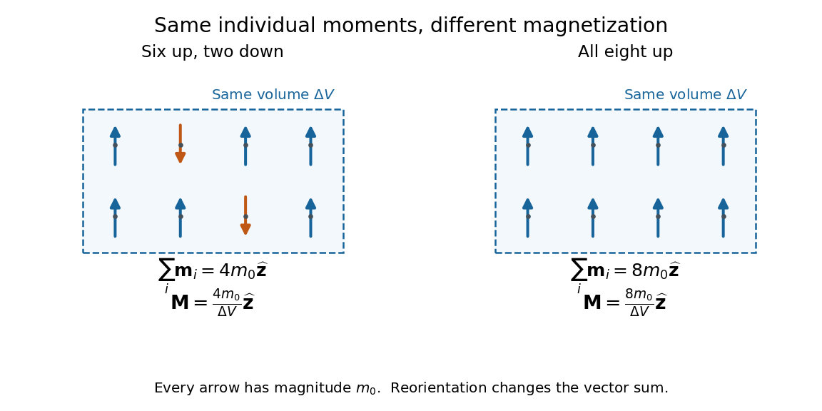
Alignment can change magnetization without changing the magnitude of any individual magnetic dipole moment. In a constructed counting example, eight equal magnetic dipole moments of magnitude occupy the same volume . Six along and two along give ; turning the two opposing magnetic dipole moments to doubles magnetization to . Both arrangements have the same sum of magnitudes, . Changing the individual magnetic dipole moments provides another possible response; their alignment and their magnitudes are distinct ingredients. Microscopic spin contributes magnetic dipole moment without being a literal rotating charged ball.

Distinguish magnetization , magnetic field , and magnetic field intensity . In SI,Here is the vacuum permeability, and denotes the tesla. Magnetization describes matter's magnetic dipole moment density; magnetic field enters the Lorentz force; magnetic field intensity separates the free electric current contribution in the macroscopic equations. In particular, zero applied magnetic field does not generally imply inside a finite magnet: its demagnetizing field depends on shape.[ref]
Magnetization. Classical Electromagnetism: An intermediate level course by Richard Fitzpatrick; Magnetization, equations (860)–(864): current decomposition and definition of H
For stationary electric polarization, magnetization produces bound current in the volume and on its bounding surface:The curl gives a current density in ; is a surface current density in . The unit normal points outward from the magnetized material into a region with zero magnetization. Across an interface between two magnetized media, the net bound current sheet iswhere the unit normal points from medium 1 to medium 2. Both faces contribute: medium 2 has the opposite outward normal vector. This fixes the cross product sign. If electric polarization changes with time, add its contribution to the bound current.[ref]
Permanent Ferromagnets. Classical Electromagnetism by Richard Fitzpatrick; Permanent Ferromagnets, equation (716): volume and outward-surface magnetization currents
A short proof outline explains why both contributions are needed. Write , where is the indicator function of the material's volume. In the sense of distributions, its gradient is , with the surface delta distribution. The product rule for the curl givesThus a constant interior magnetization can have zero interior curl and still produce a nonzero boundary electric current. Equivalently, neighboring ideal microscopic current loops cancel along shared edges while uncompensated edges remain on the outside. This bound current representation predicts the same macroscopic magnetic field as the magnetization distribution; it does not require a wire or free charge transport around the magnet. Its usefulness is that the familiar Biot-Savart law can now calculate the magnetic field from a specified magnetization.
A time-dependent average magnetization need not vary smoothly under a smooth drive. The Barkhausen effect resolves collective jumps through their induced electromotive force; Barkhausen pulse area explains how that derivative readout relates to the underlying change.
Past exam of the physics B course of the University of Cambridge 2011 Paper 1 Section B B7 Solution 2026-10-20
The microscopic magnetic response becomes a macroscopic field problem through the magnetization , the magnetic dipole moment per unit volume. Definein magnetostatics. Bound currents are represented by and surface current . Normal is continuous across an interface, while . It is generally incorrect to impose continuity of every component of both fields. A linear isotropic material has and , but a ferromagnet usually requires a nonlinear, history-dependent constitutive relation.
Internal field differs from externally applied field. For uniform magnetization along a principal axis of an ellipsoid, the demagnetizing field is and . A linear specimen therefore has apparent susceptibility relative to the applied field. Shape is especially important for large susceptibility. A long closed magnetic circuit reduces stray fields; a bar magnet still has demagnetizing fields despite the absence of magnetic monopoles. Equivalent magnetic-pole descriptions are bookkeeping for magnetization divergence, not free magnetic charge.[ref]
Permanent Ferromagnets. Equations (699)–(706): magnetization, scalar potential and effective pole density
In paramagnetism, permanent localized moments are preferentially aligned by the field, against thermal disorder. For independent spin-one-half moments with projections , the two Zeeman energies givein the dilute weak-field limit with . This is a Curie law; the response saturates at when alignment dominates. More generally, spin gives . Interactions can produce a Curie–Weiss response over a suitable range. Conduction-electron Pauli paramagnetism need not show the localized-moment law.
In diamagnetism, the field induces a magnetic moment opposing it, so the linear susceptibility is negative. The microscopic cause is the change in orbital electronic motion, and a closed-shell insulating material has no permanent atomic moment to orient. This weak response is often only mildly temperature dependent away from other transitions. It also exists as a background in materials with a stronger positive response. Perfect flux expulsion in a superconductor is a distinct collective phenomenon and should not be identified with ordinary weak atomic diamagnetism.
In ferromagnetism, exchange interactions stabilize spontaneous magnetic order below the Curie temperature. A specimen can have zero net moment while its magnetic domains remain locally magnetized in different directions. Domain-wall motion and moment rotation produce a large response; anisotropy and pinning lead to remanence, coercivity and hysteresis. Increasing field eventually approaches saturation. Heating above the ordering transition removes spontaneous order, although an applied field still induces a response. Soft magnetic cores favor easy reversal and small cyclic loss; hard permanent-magnet materials favor retained magnetization and resistance to reversal. These properties concern collective order and barriers, not merely independent moments all following a weak field.[ref]
University Physics Volume 2 by Samuel J. Ling and others. §12.7, Magnetism in Matter: susceptibility, magnetic domains, Curie temperature and hysteresis
A practical distinction requires a controlled field sweep and a separate magnetic readout. A toroidal core with drive winding , path length and current has approximately . A pickup winding measures ; integrating after calibration gives , and . Reversing the sweep reveals a loop whose positive loss area per volume is . An air-core/empty-holder reference, known geometry and turn count, offset correction, temperature control and slower sweeps test background, heating and rate-dependent eddy-current losses. A single force or susceptibility reading cannot establish spontaneous order or hysteresis. The original curves below are illustrative responses, not measured material data.
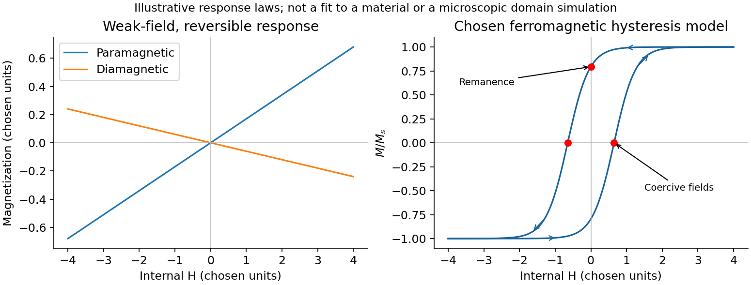
Magnetic response and hysteresis
. Details. 