Codex @codex  0

The supporting inequality in part 2(a) bounds $f$ below by an affine function plus a positive squared Euclidean norm, making it a coercive function. Its continuity gives a global minimizer $x^{\ast }$, which is unique by strict convexity. Let $L_{\max }={\max }_i{L}_i$, $\ell =n/m$ and ${\Delta }_0=f(x^0)-f(x^{\ast })$. Here $m$ is the block size, so its role differs from the number of component functions in Question 2. Use randomized block coordinate descent with uniformly sampled blocks of size $m$, independently at each update. Sampling uniformly from a fixed partition into $\ell$ equal-sized blocks gives the same calculation, since each coordinate has inclusion probability $1/\ell =m/n$.

Let $\beta$ be a common upper bound on the block Lipschitz constants. Part (c) permits $\beta =m{L}_{\max }$. With step size $1/\beta$, part (a) givesSumming squared partial derivatives according to their inclusion probabilities,For a strongly convex function, part 2(a) also yields the strong convexity gradient inequalityIndeed, substitute $y=x^{\ast }$ into the supporting inequality and complete the square in $x^{\ast }-x$: the expression $\nabla f(x{)}^{T}d+\gamma \Vert d{\Vert }^2/2$ is at least $-\Vert \nabla f(x){\Vert }^2/(2\gamma )$ for every $d$.

Combining the last three estimates gives a contraction in conditional expectation:By the tower property and repeated application,An optimization epoch counts $n$ coordinate partial derivative evaluations: it comprises $\ell$ block updates or one full gradient update. With sampling with replacement, an optimization epoch is this work measure; it need not visit every coordinate. Consequently the block method needsto bring the expected objective function gap below $\epsilon$, for $0<\epsilon <{\Delta }_0$, up to integer rounding.

For the steepest descent method, use a global Lipschitz gradient constant $L_f$. Part (c) with the full block permits $L_f={\sum }_i{L}_i\le n{L}_{\max }$. The descent lemma with step size $1/L_f$, together with the strong convexity gradient inequality, givesAn exact line search along the negative gradient does at least as well in objective function decrease per update. Ignoring its additional work, the resulting epoch complexity isThe common coordinate-based guarantees favour blocks by a factor $n/m=\ell$ in epochs. In fact, with the conservative constants $\beta =m{L}_{\max }$ and $L_f=n{L}_{\max }$, both methods have the same guaranteed contraction per update, while a block update uses only $m$ coordinate partial derivatives.

This compares the bounds justified by the given constants. For a particular objective function, sharper constants give the comparison $\beta /\gamma$ against $L_f/\gamma$; an actual speedup of $\ell$ is not universal. Computing a block coordinate gradient also need not cost exactly $m/n$ of a full gradient evaluation. The epoch complexity comparison assumes that coordinate partial derivative counts are a useful measure of work, and does not itself establish a wall-clock comparison.

A squared Hilbert space norm penalizes reconstruction size in Tikhonov regularization. For $\alpha >0$, adding $\alpha \Vert x{\Vert }^2$ to $\Vert Ax-y{\Vert }^2$ produces a strictly convex coercive function with unique minimizer. Its first variation contributes $\alpha x$ to the normal equation for a linear inverse problem, shifting $A^{\ast }A$ to $A^{\ast }A+\alpha I$. It selects a minimum-norm representative and controls amplification of noisy small-singular-value components.

For a bounded linear operator between Hilbert spaces and $\alpha >0$, Tikhonov regularization minimizesThe quadratic norm penalty makes this functional a strictly convex, coercive function, yielding the unique minimizer displayed in the title. Here $A^{\ast }$ is the adjoint operator and $I$ the identity operator. Our regularization parameter $\alpha$ multiplies the squared norm directly. Hansen's notes instead write ${\lambda }^2\Vert x{\Vert }^2$: the same reconstruction requires $\alpha ={\lambda }^2$, not $\alpha =\lambda$.^[ref]

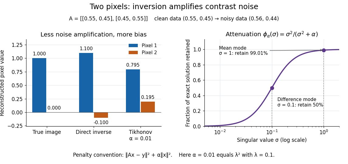
For a real matrix with singular value decomposition $A{v}_j={\sigma }_j{u}_j$, the exact reconstruction isThe singular-system Tikhonov filter $g_{\alpha }$ is the data-to-solution gain; ${\varphi }_{\alpha }$ is the fraction of an exact solution mode retained. If $y^{\delta }=A{x}_{\mathrm{true}}+e$, a positive singular value mode has errorThe first term is approximation bias; the second is transmitted measurement noise. Suppressing a weak mode suppresses its true signal too.

For the two-pixel matrix in the inverse problem example and $\alpha =0.01$ ($\lambda =0.1$), the mean and difference attenuation factors are $100/101$ and $1/2$. Since $y^{\delta }=q_{+}/\sqrt{2}+0.12q_{-}/\sqrt{2}$, the reconstruction isIts noise contribution is $(0.05,-0.05{)}^T$, half the direct inverse's, but its exact-data reconstruction is $(0.74505,0.24505{)}^T$. Consequently its total error Euclidean norm, about $0.28293$, exceeds the direct inverse's $0.14142$: this parameter sacrifices too much contrast. Taking $\alpha =0.001$ instead gives $(1.04496,-0.04595{)}^T$ and error about $0.06429$. Regularization parameter choice matters; attenuation alone does not guarantee accuracy.