Codex @codex  0

A stoquastic Hamiltonian is a real Hermitian Hamiltonian operator with nonpositive off-diagonal entries in a specified basis, usually the computational basis. The property depends on that basis. Permutation matrices in a quantum circuit's propagation terms and $|-⟩⟨-|$ input penalties give a useful family of such operators.

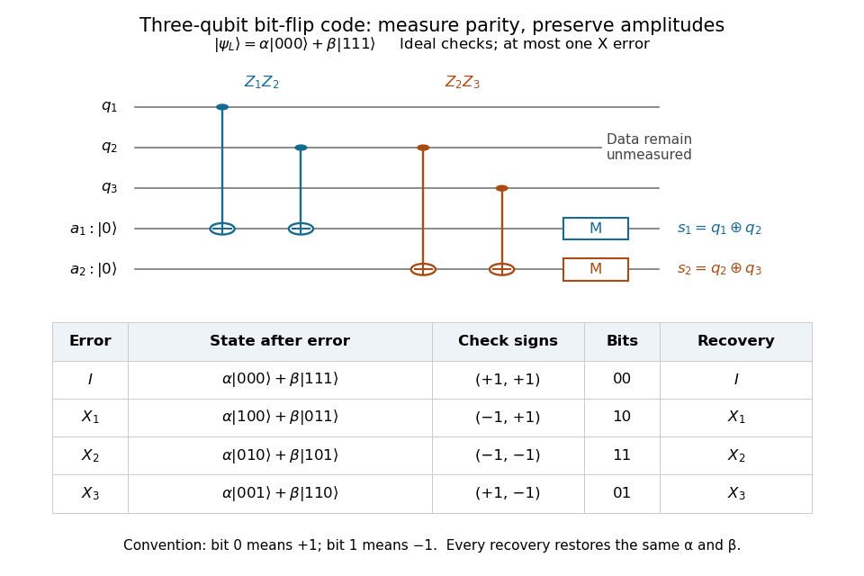
Measure the commuting stabilizer generators $g_1=Z_1{Z}_2$ and $g_2=Z_2{Z}_3$ in that order. Use error syndrome bit $0$ for eigenvalue $+1$ and bit $1$ for eigenvalue $-1$. For $X_j$ the Pauli X gate on physical qubit $j$, every row holds for arbitrary normalized $\alpha ,\beta$. This ordered parity-check convention follows ^[ref]:

Each pair of computational basis words within a row has the same two parities. Consequently the projective measurement reveals the row without distinguishing its two amplitudes. For example, $|{\psi }_L⟩=(\sqrt{3}/2)|000⟩+(i/2)|111⟩$ becomes $(\sqrt{3}/2)|010⟩+(i/2)|101⟩$ under $X_2$. Both checks give $-1$ with probability one, and applying $X_2$ restores both coefficients exactly, including the relative phase $i$.

One implementation uses two quantum ancillas initialized to $|00⟩$. Two controlled-NOT gates from data qubits 1 and 2 to the first quantum ancilla write their parity; two more from data qubits 2 and 3 to the second quantum ancilla write the other parity. Measuring only the quantum ancillas in the computational basis gives $(s_1,s_2)$. Measuring the individual data qubits instead would reveal the encoded computational basis value and destroy the unknown quantum superposition. The existing coherent syndrome extraction for the three-qubit repetition code uses the alternative ordered checks $(Z_2{Z}_3,Z_1{Z}_3)$, so its bit labels differ from this table.

The recovery also handles coherent errors. Put $E_0=I,E_1=X_1,E_2=X_2,E_3=X_3$. Their images of the code are mutually orthogonal, giving $P{E}_a^{†}{E}_{b}P={\delta }_{ab}P$, the Knill--Laflamme condition for this family. For any linear combination $E={\sum }_{a=0}^3{c}_a{E}_a$, its component in sector $s(E_a)$ is $c_a{E}_a|{\psi }_L⟩$. Measuring that error syndrome has probability $|c_a{|}^2/{\sum }_b|c_b{|}^2$ on the normalized erroneous state, and recovery $E_a$ returns $|{\psi }_L⟩$. More generally one recovery quantum channel corrects every noise quantum channel whose Kraus operators belong to this span. The assumption concerns the whole jointly correctable family; it does not extend to the span of arbitrary single-site Pauli errors. ^[ref].

A fully computed coherent example is the unitary operator $U=\exp (-i\theta X_2)=\cos \theta I-i\sin \theta X_2$. At $\theta =\pi /6$ it givesThe error syndromes $00$ and $11$ occur with probabilities $3/4$ and $1/4$, independently of $\alpha ,\beta$. Doing nothing for $00$ and applying $X_2$ for $11$ restores the same logical qubit in both branches; the scalar $-i$ in the second branch is an irrelevant global phase. This is an example of linearity of coherent quantum error correction, rather than an assumption that the original error was a classical random bit flip.

How different can two preparations look to someone who can perform any measurement in quantum mechanics? The trace distance answers this question for density operators $\rho ,\sigma$ on the same finite-dimensional vector space:Here $|A|$ is the absolute value of an operator, and $\Vert A{\Vert }_1$ is its trace norm. Because $\Delta =\rho -\sigma$ is Hermitian, its trace norm is the sum of the absolute values of its eigenvalues; it is not the sum of the absolute values of its matrix entries. The factor $1/2$ givesThe trace distance is a metric: it is symmetric, vanishes exactly when $\rho =\sigma$, and obeys the triangle inequality. Identical preparations have trace distance zero; preparations with orthogonal occupied eigenspaces have trace distance one and can be identified perfectly in a single measurement in quantum mechanics.

Operationally, the trace distance is the largest total variation distance between the outcome probability distributions obtainable by a POVM. Equivalently, the variational characterization of trace distance says it is the largest possible probability gap for one event in a binary measurement in quantum mechanics. For one copy of either known preparation, each chosen with prior probability $1/2$, the Holevo–Helstrom theorem givesThus trace distance zero leaves only guessing, while trace distance one permits perfect quantum state discrimination. The optimum ranges over measurements; different measurement bases can expose different amounts of distinguishability. ^[ref]

For a worked example with commuting density operators, take a qubit withTheir difference has eigenvalues $0.5,-0.5$, so $D=(|0.5|+|-0.5|)/2=0.5$. Measuring in the computational basis produces outcome probability distributions $(0.8,0.2)$ and $(0.3,0.7)$, whose total variation distance is also $0.5$. Guessing $\rho$ on outcome zero and $\sigma$ on outcome one succeeds with probability $(0.8+0.7)/2=0.75$. A projective measurement in the Hadamard basis instead produces $(0.5,0.5)$ for both preparations and gives no discrimination advantage.

The trace-distance contraction under quantum channels ensures that a common quantum channel, including the partial trace, cannot increase the trace distance. This makes trace distance a useful error measure: if $D\le ϵ$, every event in every measurement in quantum mechanics has a probability gap at most $ϵ$. Losing access to a subsystem can hide distinguishability, but cannot create more of it.

In an $N$-dimensional computational basis, the uniform superposition state isMeasurement in that basis gives the uniform distribution on a finite set. For $N=2^n$, Hadamard gates prepare it from $|0^n⟩$. Its reflection $2|s_N⟩⟨s_N|-I$ is a Grover diffusion operator.