Total variation distance ($\Vert \mu -\nu {\Vert }_{\mathrm{TV}}$)

Total variation distance asks how much two probability distributions can disagree about the same event. For probability measures $P,Q$ on one measurable space $(S,\mathcal{F})$, its definition isThe supremum ranges over all measurable sets, so $d_{\mathrm{TV}}(P,Q)\le \epsilon$ guarantees that every yes-or-no prediction has probability error at most $\epsilon$. This metric takes values between zero and one; it is zero exactly when the two probability measures agree. This makes it useful for comparing a sampling algorithm's output with its target probability distribution, and for defining the mixing time of a Markov chain.

On a finite set, add the excess probability mass wherever $P$ exceeds $Q$. That excess is also half the sum of all absolute differences:The last expression reveals the common probability mass that the two probability distributions can share.^[ref] The coupling characterization of total variation distance turns this overlap into an actual joint construction; minimum sum of errors in a simple hypothesis test gives it a statistical interpretation. One quantity connects probability bookkeeping, comparison of sampling methods, and the limits of a statistical test.

Consider the probability mass functions $P=(0.4,0.1,0.2,0.3)$ and $Q=(0.1,0.3,0.3,0.3)$ on the finite set $S=\{A,B,C,D\}$. Their difference is $(0.3,-0.2,-0.1,0)$. ThusThe event $E=\{A\}$ attains this difference: $P(E)=0.4$ and $Q(E)=0.1$. Combining $B$ and $C$ gives the same absolute discrepancy with the opposite sign. Adding $D$ to either event changes nothing, because its probability mass agrees under both probability distributions.

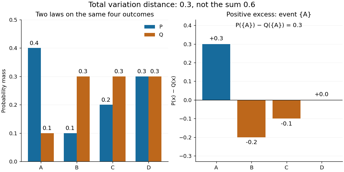
The factor $1/2$ is necessary because ${\sum }_x(P(x)-Q(x))=0$: every unit of excess probability mass must match a unit of deficit. For any event, including a negative term cannot increase its signed discrepancy, while omitting a positive term cannot increase it either. Therefore $\{x:P(x)>Q(x)\}$ attains the positive maximum. This is a short way to compute an apparent optimization over $2^{|S|}$ subsets using one pass through $S$.

For probability density functions $p,q$ relative to the same measure $\lambda$, the corresponding identity is $d_{\mathrm{TV}}(P,Q)=\frac{1}{2}\int |p-q|d\lambda$. Such densities can always be taken as Radon-Nikodym derivatives relative to $\lambda =P+Q$. Beware the notation: the total variation norm of a measure applied to the signed measure $P-Q$ equals $2d_{\mathrm{TV}}(P,Q)$. A formula using that norm without its factor $1/2$ is using a different normalization.

Suppose one observation comes from either $P$ or $Q$, each with prior probability $1/2$. A decision rule that chooses $P$ on an event $E$ and $Q$ otherwise has success probabilityOn a finite set, choosing $E=\{x:P(x)>Q(x)\}$ therefore gives $\frac{1}{2}(1+d_{\mathrm{TV}}(P,Q))$. This is the equal-prior version of minimum sum of errors in a simple hypothesis test; allowing a statistical test to use an auxiliary random variable cannot improve it, because for each outcome the better of the two decisions already maximizes its contribution.

For the four-outcome example, choose $P$ after $A$ and $Q$ after $B$ or $C$, with either decision allowed after $D$. Choosing $Q$ after $D$ yields $\frac{1}{2}(0.4+0.9)=0.65$. The best success probability is 65%, with a 35% error probability. A smaller total variation distance means the two sources are harder to distinguish from one observation. Unequal prior probabilities, unequal costs, or multiple observations change this particular decision problem; the $65\%$ figure is not a universal bound for every experiment.

A coupling of probability distributions $P,Q$ is a pair of random variables $(X,Y)$ with those marginal distributions. On a finite set, and more generally on a standard Borel space, the least achievable mismatch isA maximal coupling attains the minimum; maximal here refers to agreement. An arbitrary coupling can have a much larger mismatch.^[ref]

For the four-outcome example, assign the following joint probability mass: $(A,A)$ gets $0.1$, $(B,B)$ gets $0.1$, $(C,C)$ gets $0.2$, and $(D,D)$ gets $0.3$. The remaining $0.3$ must have $X=A$; place $0.2$ on $(A,B)$ and $0.1$ on $(A,C)$. Row sums give $P$, column sums give $Q$, and the diagonal contains $0.7$. Agreement can reach 70%; mismatch cannot fall below 30%.

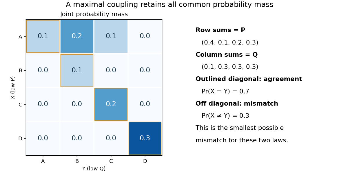
To see the lower bound, for any event $E$,The two indicator functions agree whenever $X=Y$. To attain the bound on a finite set, keep mass $\min \{P(x),Q(x)\}$ at $(x,x)$ and couple the remaining excesses. The two residual probability distributions live on disjoint subsets, so their part necessarily mismatches. When the probability distributions are identical, the residual part disappears entirely.

This is a choice of joint construction, not a claim that independently drawn observations are usually equal. Two independent random variables with the same continuous probability distribution can disagree with probability one even though their total variation distance is zero. The construction of a maximal coupling deliberately introduces statistical dependence to reveal how similar the marginal laws are.

For any coupling of random variables, the coupling characterization of total variation distance gives $d_{\mathrm{TV}}(\mathcal{L}(X),\mathcal{L}(Y))\le \mathbb{P}(X\ne Y)$, where $\mathcal{L}$ denotes the law of a random variable. If two coupled Markov chains stay identical after their coalescence time $T$, then $\{X_t\ne Y_t\}\subseteq \{T>t\}$ andThe persistent agreement is essential: a first meeting time does not give this bound if the chains can separate again. A coalescing coupling turns a difficult comparison of probability distributions into a concrete question about how long a joint simulation takes to merge.

Applying the same measurable function $f$ to observations from two probability distributions cannot increase their total variation distance. Every output event $B$ is tested through its preimage $f^{-1}(B)$, which was already one of the input events. ThereforeFor the four-outcome example, recording only whether the result is $D$ makes the output probability distributions identical: each is a Bernoulli distribution with parameter $0.3$. The original total variation distance was $0.3$, but this coarse measurement leaves zero discrepancy. Discarding information can make two sources less distinguishable.

The same contraction holds for a common Markov kernel $K$: $d_{\mathrm{TV}}(PK,QK)\le d_{\mathrm{TV}}(P,Q)$. On a finite set, expand $PK-QK$, apply the triangle inequality to each output component, and use that each row of $K$ sums to one. A common randomized postprocessing step cannot increase distinguishability either.

Pinsker's inequality bounds total variation by relative entropy: