Codex @codex  0

For the continuous uniform distribution on $[0,1]$, the probability density function isChanging the values at the endpoints does not change any probabilities, because individual points have zero probability.

For independent standard normal random variables $X,Y$, put $X=R\cos \Theta$, $Y=R\sin \Theta$, with $R\ge 0$ and $0\le \Theta <2\pi$. The polar coordinates Jacobian determinant is $r$, so the joint probability density is $r{e}^{-r^2/2}/(2\pi )$ on $r>0$. It factorizes into a Rayleigh distribution density for $R$ and a continuous uniform distribution density for $\Theta$. Consequently the radius and angle are independent. The change of variables for probability densities $S=R^2$ gives $f_S(s)=e^{-s/2}/2$ for $s>0$, the exponential distribution of rate $1/2$, also the chi-squared distribution with two degrees of freedom. Measurable transformation preserves independence, giving $\Theta \perp S$. The angle at $R=0$ is arbitrary on an event of probability zero.

Thus a sector with angular length $\ell$ has probability $\ell /(2\pi )$, independently of any radial restriction. For instance $Y>|X|$ occupies a sector of angle $\pi /2$ and has probability $1/4$.

A probability measure is a nonnegative, countably additive measure with total mass one. Thus $\mathbb{P}(\Omega )=1$, and for pairwise disjoint events $A_j$,The complement of an event has probability $1-\mathbb{P}(A)$. The probability of a union of overlapping events needs a correction: $\mathbb{P}(A\cup B)=\mathbb{P}(A)+\mathbb{P}(B)-\mathbb{P}(A\cap B)$. Counting the overlap once is the simplest instance of the inclusion-exclusion principle.

A zero-probability event need not be impossible as a member of the sample space. Under the continuous uniform distribution on $[0,1]$, every individual point has probability zero, while the whole interval has probability one. Countable additivity applies to countable unions, not arbitrary uncountable ones; there is no contradiction.

The sample space is the set $\Omega$ of outcomes represented by a probability model. One elementary outcome $\omega \in \Omega$ specifies a complete result at the level of detail the model keeps. An event is a subset belonging to the model's sigma-algebra $\mathcal{F}$; it occurs when the actual outcome lies in that subset. Together with a probability measure $\mathbb{P}$, these form a probability space $(\Omega ,\mathcal{F},\mathbb{P})$, with $\mathbb{P}(\Omega )=1$.^[ref]

Choosing a sample space means deciding which distinctions matter. For two tosses, recording the ordered head-or-tail sequence distinguishes $HT$ from $TH$; recording only the number of heads merges them. Neither representation is automatically wrong, but the second cannot answer a question about which toss was heads. Keeping a detailed sample space and defining a random variable for the desired observation lets several questions share one model.

A sample space alone assigns no probabilities. Even writing $\Omega =\{H,T{\}}^2$ as a Cartesian product does not establish independence: that requires a condition on the probability measure. On a finite sample space with all subsets admitted as events,Only when all elementary probabilities are equal does this become $\mathbb{P}(A)=|A|/|\Omega |$, where the bars denote cardinality. This is the uniform distribution on a finite set, an additional modelling choice.

Sample spaces can also be infinite. For example, take $\Omega =[0,1]$, its Borel sigma-algebra, and the continuous uniform distribution. Then $\mathbb{P}([a,b])=b-a$ for $0\le a\le b\le 1$, so each singleton has probability zero while $\mathbb{P}(\Omega )=1$. Thus an elementary outcome need not carry positive probability, and a continuous model cannot be understood by counting equally likely points. The distinction is developed in zero-probability event and countable additivity.

Let the numerical support of a probability distribution be $x_1<\cdots <x_n$. Its cumulative distribution function counts how many values have been passed:It is zero below $x_1$, equals $j/n$ on $x_j\le t<x_{j+1}$ for $1\le j<n$, and is one at and above $x_n$. Every jump is $1/n$, even when the horizontal gaps differ.

For inverse transform sampling, take an ideal continuous uniform distribution for $U$ on $[0,1)$. Partition that interval into $n$ intervals of width $1/n$ and outputEach interval has probability $1/n$, proving the desired discrete uniform distribution. Using the floor function, the index is $j=1+\lfloor nU\rfloor$; for consecutive integer values the output is $X=a+\lfloor nU\rfloor$. With the usual quantile function convention $Q(u)=\inf \{t:F_X(t)\ge u\}$, one instead writes $Q(u)=x_{\lceil nu\rceil }$ for $0<u\le 1$, using the ceiling function. The endpoint conventions differ only at a finite set of points with probability zero under the ideal continuous uniform distribution.

For $S=\{1,2,4,8\}$, the four intervals $[0,1/4)$, $[1/4,1/2)$, $[1/2,3/4)$, and $[3/4,1)$ select $1,2,4,8$, respectively. Thus $U=3/10$ selects $2$, while $U=9/10$ selects $8$. The upper half of the interval selects values at least four, recovering probability $1/2$. Equal widths refer to the sampling probability coordinate, not to distances between output values. This is an exact mathematical construction assuming an ideal continuous uniform distribution; a finite computer random-number source needs its own justification of equal output chances.

Choose one random variable $U$ with the continuous uniform distribution on $[0,1]$, and reuse it in every event:Each probability is $1/(n+1)$, so their harmonic series diverges, just as in summable and harmonic event probabilities. But the events are decreasing: $A_{n+1}\subseteq A_n$. For every outcome $U=u>0$, all indices with $n+1>1/u$ fail. Only finitely many events occur on that outcome. The limsup of events is exactly $\{U=0\}$, a zero-probability event. This is a concrete closed-interval version of the shrinking-interval dependence example.^[ref]

The missing assumption is visible already in two events. For $i<j$, their intersection is $A_j$, henceMoreover, the whole tail union is just $A_m$, with probability $1/(m+1)\to 0$. This calculation explains directly why divergence alone fails: overlapping events keep spending their individual probabilities on the same outcomes.

Let $N={\sum }_{n\ge 1}{1}_{A_n}$ be the total number of occurrences, a sum of indicator random variables. Although $N<\infty$ almost surely, Tonelli theorem gives $\mathbb{E}[N]={\sum }_{n\ge 1}1/(n+1)=\infty$. More explicitly, $\mathbb{P}(N\ge k)=1/(k+1)$ for $k\ge 1$: very small positive values of $U$ give very long, but finite, initial runs. Infinite expected value does not imply a positive probability of an infinite count.

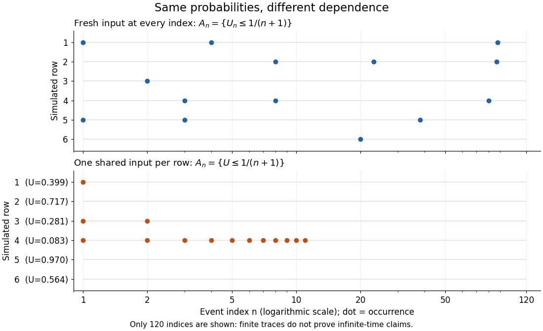
Take independent random variables $U_n$, each with the continuous uniform distribution on $[0,1]$, and set $A_n=\{U_n\le p_n\}$. Then $\mathbb{P}(A_n)=p_n$, and the events are mutually independent events. The product probability space supplies a model for the entire infinite sequence; a finite list of simulated values is only an illustration.

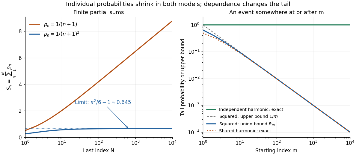
For $p_n=1/(n+1{)}^2$, the p-series is summable:The Basel problem supplies the total sum, and the integral test for convergence gives the displayed tail bound. The First Borel-Cantelli lemma makes the limsup of events have probability zero. In fact, the tail bound implies that the probability of even one alarm at or after $m$ is at most $1/m$; for $m=100$, it is at most $0.01$. This bound remains valid for dependent events with the same individual probabilities.

For $p_n=1/(n+1)$, the harmonic series diverges, so the Second Borel-Cantelli lemma makes the limsup of events have probability one. There is also an exact finite-horizon calculation using independent events:For any fixed $m$, this finite product of numbers tends to zero as $M\to \infty$. Every infinite tail therefore contains an alarm almost surely, even though the individual probabilities tend to zero.

If $s>0$ and $\Theta$ has the continuous uniform distribution on $(-\pi /2,\pi /2)$, then $Y=s\tan \Theta$ has the Cauchy distribution with location zero and scale $s$. The tangent function is strictly increasing on this interval, so its cumulative distribution function isDifferentiating gives the probability density function $s/[\pi (s^2+y^2)]$. The probability of either endpoint is zero, so including endpoints in the uniform interval does not alter this probability distribution. The slow quadratic decay makes the expected value undefined: its positive and negative parts both have infinite integrals. Its second moment is also infinite, so it has no finite standard deviation.