Codex @codex  0

For an absolutely continuous $f$ with $f(0)=0$, this causal Abel integral equation has inversionUnder Laplace-transform growth hypotheses, the convolution theorem for Laplace transforms converts the original kernel into $\Gamma (1-\alpha )s^{\alpha -1}$. Since $\mathcal{L}[f^{\prime }]=s\mathcal{L}[f]$, the transformed inverse is $s^{-\alpha }\mathcal{L}[f^{\prime }]/\Gamma (1-\alpha )$, giving the formula. It also holds locally in the corresponding integrable convolution class: convolving the two power kernels produces the constant $B(\alpha ,1-\alpha )=\Gamma (\alpha )\Gamma (1-\alpha )$ by the beta-gamma identity, so substitution recovers ${\int }_0^t{f}^{\prime }=f(t)$. The same convolution identity proves uniqueness in that class. For example $f(t)=t$ gives $\Phi =t^{\alpha }/[\Gamma (\alpha +1)\Gamma (1-\alpha )]$.

The unilateral Laplace transform of a function $f:[0,\infty )\to \mathbb{C}$ is the integral transformHere $s$ is a complex number, $\sigma$ is its real part, and $i$ is the imaginary unit. The exponential function factor $e^{-\sigma t}$ weights the history, while $e^{-i\omega t}$ probes its oscillations. The integral starts at zero, so it uses only the history from that starting time onward. This section concerns ordinary functions; their value at the single endpoint does not change the integral. See MIT 18.03SC, definition and elementary examples.

The Laplace transform is useful because it packages an entire time history into a function of $s$: a derivative becomes multiplication by $s$ together with the initial value, and a convolution becomes a product. Thus a linear differential equation can become an algebraic equation that already remembers its initial value problem. The worked example below shows both descriptions of the same response.

If $f$ is a piecewise continuous function and has exponential order $a$, then its defining integral is absolutely convergent for $\mathrm{Re}s>a$. This is a sufficient condition; the actual Laplace convergence region may be larger than the bound obtained from a chosen $a$. ^[ref].

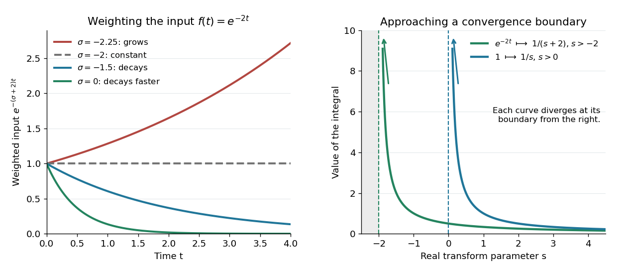
The bound has a short explanation. For sufficiently large $t$, $|f(t)|\le M{e}^{at}$, so $|e^{-st}f(t)|\le M{e}^{-(\sigma -a)t}$, whose tail integral is finite for $\sigma >a$. The finite initial interval is covered by piecewise continuity.

Three calculations make the convergence condition concrete. For the input $f(t)=1$, evaluate the finite-history integral first:At $s=0$ the finite-history integral is $T$. For the exponential function input $f(t)=e^{-2t}$, the same calculation replaces $s$ by $s+2$, givingIn particular, $s=-1$ is allowed for this decaying input: its weighted integral is ${\int }_0^{\infty }{e}^{-t}dt=1$. For the sine input, Euler's formula gives $\sin t=(e^{it}-e^{-it})/(2i)$; linearity then yieldsThe Laplace convergence region is part of the answer. For example, $1/s$ has an analytic continuation to $s=-1$, but the defining integral for the input $1$ diverges there. The sine calculation is also developed in MIT 18.03SC, further elementary transforms.

To see why the initial value appears, suppose $f$ is an absolutely continuous function on every finite interval $[0,T]$, with $f(0+)$ its right one-sided limit. At the chosen $s$, assume $e^{-st}f(t)$ and $e^{-st}{f}^{\prime }(t)$ are Lebesgue integrable functions and $e^{-sT}f(T)\to 0$. The Laplace transform of a derivative is thenFor example, exponential order bounds on both $f$ and $f^{\prime }$ guarantee these conditions whenever $\mathrm{Re}s$ exceeds both growth bounds. The initial value is the lower-end boundary contribution of integration by parts.

Consider the initial value problemWrite $Y=\mathcal{L}\{y\}$. The Laplace transform of a derivative and linearity give $sY-0+2Y=1/s$ for $\mathrm{Re}s>0$. A partial fraction decomposition therefore givesWe recognize the two elementary Laplace transforms already computed. Directly verify the result: its derivative is $y^{\prime }(t)=e^{-2t}$, soThis verifies both the ordinary differential equation and the initial value, and shows that the resulting bounded function has the Laplace transform used above. The response rises from zero toward $1/2$: at that value the input $1$ balances the term $2y$. The general method is described in MIT 18.03SC, solving initial value problems.

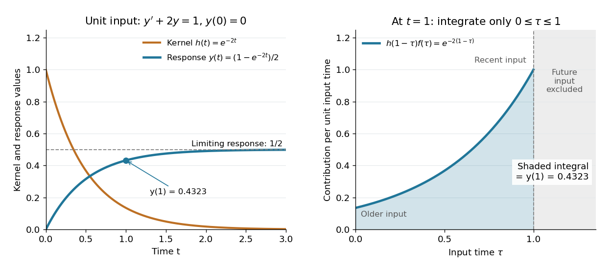
The same solution is a convolution. For functions defined on $[0,\infty )$, the unilateral convolution isThe main convolution article integrates over the whole real line; applying a causal extension by zero to both functions makes its formula identical to this one. Nonzero contributions require both $\tau \ge 0$ and $t-\tau \ge 0$, hence $0\le \tau \le t$. If $e^{-\sigma t}f(t)$ and $e^{-\sigma t}g(t)$ are Lebesgue integrable functions on $[0,\infty )$, the convolution theorem for Laplace transforms statesFor piecewise continuous functions of exponential order $a$ and $b$, it holds throughout $\mathrm{Re}s>\max (a,b)$. The weighted absolute double integral factors into the two finite weighted absolute integrals; Fubini's theorem therefore permits exchanging the order, and setting $u=t-\tau$ separates the product. ^[ref].

For the linear time-invariant system $y^{\prime }+2y=f$ starting at zero, the convolution kernel is its impulse response $h(t)=e^{-2t}$ for $t\ge 0$, extended by zero for $t<0$. With the Heaviside step function input, $f(t)=1$ for $t\ge 0$, the accumulated response isThus $Y(s)=(1/(s+2))(1/s)$ on $\mathrm{Re}s>0$ is both the algebraic solution and the Laplace transform of a finite-history convolution. Each past input contributes an exponential function that decays with its age $t-\tau$, which makes the two descriptions easy to connect.

Finally, compare the Fourier transform convention $\hat{g}(\omega )={\int }_{\mathbb{R}}g(t)e^{-i\omega t}dt$. If $f_0$ is the causal extension by zero of $f$, define $g_{\sigma }(t)=e^{-\sigma t}{f}_0(t)$. Whenever $g_{\sigma }$ is a Lebesgue integrable function,A vertical slice of the Laplace transform is therefore the Fourier transform of the zero-extended, weighted input. Positive $\sigma$ damps its positive-time history. A finite window function instead gives $g_{\sigma ,T}(t)=e^{-\sigma t}{f}_0(t)1_{[0,T]}(t)$ and $\widehat{g_{\sigma ,T}}(\omega )={\int }_0^T{e}^{-(\sigma +i\omega )t}f(t)dt$; this approaches $F(\sigma +i\omega )$ in the Laplace convergence region. Setting $\sigma =0$ directly requires an integrable zero-extended input: the input $1$ fails that condition, even though its Laplace transform exists for every $\sigma >0$.

The history of the Laplace transform spans several stages. Schiff's historical summary notes that Laplace's 1812 treatise acknowledged earlier work on integral transforms and describes later development of the modern Laplace transform method. ^[ref].

Assume the Laplace integrals converge absolutely in a common right half-plane. The Fubini theorem and the substitution $t=u-v$ on $u\ge v\ge 0$ give the convolution theorem for Laplace transforms:For the specified inverse-square-root function, the supplied identity says $f\ast f=\pi$ on $t>0$. Consequently $\hat{f}(p{)}^2=\pi /p$. For real $p>0$ the defining integral is positive, fixing the positive square root; analytic continuation into $\mathrm{Re}p>0$ giveswith the branch positive on the positive real axis. The square identity alone would not select the sign.

Part (i) gives $\mathcal{L}(t)=1/s^2$ and $\mathcal{L}(t{e}^{-t})=1/(s+1{)}^2$. The convolution theorem for Laplace transforms therefore givesRepeated integration by parts yieldsSubstitution gives $f(t)=t-2+(t+2)e^{-t}$, agreeing with the contour integration result.

Use the printed coordinate derivative $u_x(0,t)$, not an outward normal derivative; at the left endpoint these have opposite signs. Assume the usual bounded or admissibly growing solution at infinity, with an initial trace $b_0=u_0(0)$ and forcing possessing a Laplace transform. Set $a=\alpha /2$, so $\beta =a^2$, and use $z=\sqrt{p}$ on the principal square root branch. DefineThe half-line Dirichlet Green function for $p-{\partial }_x^2$ givesWrite the transformed solution as $U=U_D+e^{-zx}B(p)$. The Laplace transform of a derivative in the dynamic boundary condition is $pB-b_0$, soThe special choice of $\beta$ gives the perfect squareIn particular, the initial boundary trace cannot be omitted. Withan integral representation isChoose the Bromwich contour to the right of the forcing's growth abscissa and every pole; $\gamma >\max (0,a^2)$ and sufficiently large for the data is a safe choice for real $a$. No sign of $\alpha$ is explicitly imposed in this question.

The inverse transform can also be performed explicitly. For the repeated-root dynamic-boundary heat kernel, setFirst integrate the Heat Poisson kernel against $e^{ar}$, or differentiate the result with respect to $a$:Since differentiation of $(\sqrt{p}-a{)}^{-1}$ with respect to $a$ produces $(\sqrt{p}-a{)}^{-2}$, and ${\partial }_a{E}_a=(-x+2at)E_a+2\sqrt{t/\pi }{e}^{-x^2/(4t)}$, the desired kernel isHere $\mathrm{erfc}$ is the complementary error function. A direct integral characterization, also proving the sign and the transform, isThe convolution theorem for Laplace transforms now gives the fully real time-domain representationAll quantities here are known from the prescribed data. For $x>0$ it tends to $u_0(x)$ as $t\downarrow 0$. At $x=0$, $J_a(0,t)\to 1$ and the spatial correction tends to zero, recovering $b_0$. A solution classical through the initial corner additionally needs $u_0^{\prime \prime }(0)+\alpha u_0^{\prime }(0)+a^2{b}_0=f(0)$; weaker corner regularity does not invalidate the formula for positive times.

The repeated-root unstable heat boundary mode gives a useful sign check on the dynamic boundary condition for the heat equation. If $a>0$, $(\sqrt{p}-a{)}^2$ has a genuine double pole at $p=a^2$ on the physical branch, and the exact homogeneous mode $e^{-ax+a^{2}t}$ satisfies both the heat equation and the printed boundary condition. Generic data can also excite a $t{e}^{a^{2}t}$ contribution. A contour deformation must retain this repeated-pole contribution. If $a<0$, the putative root $\sqrt{p}=a$ is outside the chosen branch and is not a physical pole. At $a=0$, $J_0=\mathrm{erfc}(x/(2\sqrt{t}))$, as expected when the boundary trace satisfies $b^{\prime }(t)=f(t)$.

For causal functions the convolution is $(f\ast g)(t)={\int }_0^{t}f(\tau )g(t-\tau )d\tau$. In a half-plane of absolute convergence, changing variables $u=t-\tau$ in its Laplace transform and using Fubini's theorem givesThis proves the convolution theorem for Laplace transforms. Transforming the differential equation gives $(s^2+1)Y(s)=sy(0)+y^{\prime }(0)+F(s)$. The direct transform pairs $\mathcal{L}(\cos t)=s/(s^2+1)$ and $\mathcal{L}(\sin t)=1/(s^2+1)$ then giveFor a continuous forcing, call the last term $w(t)$. The Leibniz integral rule gives $w^{\prime }={\int }_0^{t}f(\tau )\cos (t-\tau )d\tau$ and $w^{\prime \prime }=f(t)-w(t)$. Also $w(0)=w^{\prime }(0)=0$. Thus both the original equation and the initial values hold.

For an impulse at positive time $T$, the Dirac delta evaluates the convolution, yieldingHere $H$ is the Heaviside step function. The displacement remains continuous at $T$, while its derivative jumps upward by one, exactly as required by integrating the differential equation across the unit impulse.

The one-sided Laplace transform is $\bar{f}(p)={\int }_0^{\infty }{e}^{-pt}f(t)dt$. Its Bromwich inversion formula is $f(t)=(2\pi i{)}^{-1}{\int }_{\gamma -i\infty }^{\gamma +i\infty }{e}^{pt}\bar{f}(p)dp$, with an upward vertical contour to the right of all singularities and within the appropriate convergence half-plane.

To derive the convolution theorem for Laplace transforms, transform $x(t)={\int }_0^{t}f(\tau )g(t-\tau )d\tau$. With $u=t-\tau \ge 0$, the triangular integration region becomes a quadrant. Fubini's theorem gives $\bar{x}(p)={\int }_0^{\infty }{\int }_0^{\infty }{e}^{-p(u+\tau )}f(\tau )g(u)dud\tau =\bar{f}(p)\bar{g}(p)$, under the usual absolute convergence hypotheses. Inversion gives the required convolution formula.

For the differential equation, the transformed initial conditions give $(p^2-1)\bar{y}=\bar{g}+p+1$, hence $\bar{y}=\bar{g}/(p^2-1)+1/(p-1)$. Since $\mathcal{L}[\sinh t]=1/(p^2-1)$ for $\mathrm{Re}p>1$, the convolution yieldsThe integral and its first derivative vanish at zero, so the homogeneous term supplies both initial values. Differentiating twice gives the forcing through the unit derivative of the hyperbolic-sine kernel at zero.

Treat the left side as a causal convolution with $t^{-\alpha }$. Under the usual Laplace-transform hypotheses, the convolution theorem for Laplace transforms givesFor an absolutely continuous $f$ with $f(0)=0$, the derivative transform is $\mathcal{L}[f^{\prime }]=s\hat{f}$. ConsequentlySince $\mathcal{L}[t^{\alpha -1}]=\Gamma (\alpha )s^{-\alpha }$, inverting the product provesHere $0<\alpha <1$ makes both power kernels locally integrable. For example assume exponential growth bounds sufficient for the transforms and a regularity class where the convolution is defined. This is the Abel integral equation of fractional order; the initial value removes the extra boundary term in the derivative transform.

For $f(t)=t$, the remaining integral is ${\int }_0^t(t-\tau {)}^{\alpha -1}d\tau =t^{\alpha }/\alpha$. ThusSubstitution into the original equation checks the result: scaling $\tau =tu$ gives $tB(\alpha +1,1-\alpha )/[\Gamma (\alpha +1)\Gamma (1-\alpha )]=t$ by the beta-gamma identity.

Use the causal convolution $(f_0\ast f_1)(x)={\int }_0^x{f}_0(t)f_1(x-t)dt$. The convolution theorem for Laplace transforms and (i) giveSince $\mathcal{L}(\cos x)=p/(p^2+1)$, uniqueness of the Laplace transform yieldsAt $x=0$ the right side is $1-1=0$, agreeing with the empty convolution integral. Identification of $f_0$ as a Bessel function is unnecessary.

The integral $I$ is the convolution of the positive-half-line kernels $x^{a-1}$ and $x^{b-1}$. The convolution theorem for Laplace transforms therefore gives, for $p>0$,On the other hand, the substitution $t=xu$ gives $I(x)=x^{a+b-1}B(a,b)$, where $B(a,b)={\int }_0^1{u}^{a-1}(1-u{)}^{b-1}du$ is the beta function. Applying part (i) again yields $\mathcal{L}I(p)=B(a,b)\Gamma (a+b)p^{-(a+b)}$. Comparing the two expressions provesAll integrands used in the real-$p$ convolution argument are nonnegative, so Tonelli's theorem justifies the interchange; the endpoint singularities are integrable because $a,b>0$.