Codex @codex  0

Keep baseline covariates fixed and put $q=1-\pi$, ${\mu }_j=e^{{\beta }_0+{\beta }^T{x}_i+{\alpha }_j}$, and $r=1/\tau$ for $\tau >0$. Integration of a Poisson count over the Gamma component givesThis negative binomial distribution has mean ${\mu }_j$ and variance ${\mu }_j+\tau {\mu }_j^2$. Therefore the unconditional one-term distribution is the zero-inflated negative binomial distributionIn particular its zero probability is $\pi +q(1+\tau {\mu }_j{)}^{-1/\tau }$, not simply $\pi$. As $\tau \downarrow 0$ this becomes a Zero-inflated Poisson distribution.

The mixing effect has $\mathbb{E}{b}_i=q$, $\mathbb{E}{b}_i^2=q(1+\tau )$ and $\mathrm{Var}(b_i)=q(\tau +\pi )$. The law of total variance and law of total covariance now giveEquivalently, for $\mu =({\mu }_1,{\mu }_2,{\mu }_3{)}^T$, $\mathbb{E}{Y}_i=q\mu$ and $\mathrm{Cov}(Y_i)=\mathrm{diag}(q\mu )+q(\tau +\pi )\mu {\mu }^T$. This also supplies raw second moments by adding $(\mathbb{E}{Y}_i)(\mathbb{E}{Y}_i{)}^T$. Dependence arises from both shared heterogeneity and shared structural zeros, even when the positive random effect is constant.

The printed moment variance matches the hierarchical variance at the same parameter values, but its printed off-diagonal covariance is $\tau {\mu }_j{\mu }_k$. Equality would require $\tau =q(\tau +\pi )$, or $\pi (\tau -q)=0$. It is therefore false to claim that the two approaches consistently estimate all the same parameters in general.

The precise distinction is between consistency of mean ratios and identification of structural parameters. In the hierarchical model, with $m_j=q{\mu }_j$, both the quadratic variance coefficient and the covariance coefficient in terms of the marginal mean areFor the moment parameterization, writing its parameters as ${\pi }_Q,{\tau }_Q,q_Q=1-{\pi }_Q$, these coefficients are $A_Q=({\pi }_Q+{\tau }_Q)/q_Q$ and $B_Q={\tau }_Q/q_Q^2$. Its intercept is identifiable from the mean only as ${\gamma }_{0Q}={\beta }_{0Q}+\log q_Q$. Matching the true first two moments demands $A_Q=B_Q=\kappa$. One solution always isFor $\kappa >1$ there is also a solution $q_Q=1/\kappa$, ${\pi }_Q=1-1/\kappa$, ${\tau }_Q=1/\kappa$, with the corresponding shifted intercept. Indeed eliminating ${\tau }_Q$ gives ${\pi }_Q({\tau }_Q-q_Q)=0$. This is moment aliasing in a shared zero-inflated count model: matching the moments does not identify the actual structural-zero probability.

For a concrete counterexample take $\pi =0.2,\tau =0.3$. Then $q=0.8$ and $\kappa =0.625$. The only admissible moment-matching choice is ${\pi }_Q=0,{\tau }_Q=0.625$, with an intercept shifted by $\log 0.8$; it cannot recover the true structural-zero proportion 0.2. Correct marginal means can give consistent term and baseline-covariate slopes with sandwich standard errors; they do not justify consistent estimation of the intended $\pi ,\tau$, or latent intercept. Nor does a mean-only estimating equation identify $\pi$ at all. Full-distribution inference provides information beyond these first two moments.

In the usual causal stationary convention, a centered autoregressive moving-average model satisfiesSet $\Phi (z)=1-{\sum }_{j=1}^p{\varphi }_j{z}^j$ and $\Theta (z)=1+{\sum }_{j=1}^q{\theta }_j{z}^j$. After removal of common factors, the usual causality condition is that all zeros of $\Phi$ lie outside the closed unit disk. Then $\Theta (z)/\Phi (z)$ has an absolutely summable causal coefficient sequence, giving a linear-filter representation of $X$ in terms of white noise. Invertibility of the moving-average part is a separate issue and is not needed for its covariance spectrum.

White noise has one-sided density ${\sigma }^2/\pi$. Applying the filtering result, or equating the spectra of the two filtered sides of the defining equation, givesThe moving-average sign agrees with the positive $\theta$ convention used later. More generally, the same quotient applies to a stationary two-sided solution when the reduced denominator has no unit-circle zeros; causality selects the past-dependent realization. This is the spectral density of an ARMA process.

The series defining the linear filter of a stationary time series converges in $L^2$, because the norm of a tail is at most $\Vert X_0{\Vert }_2$ times the corresponding tail sum of $|a_s|$. Its mean is the original mean times ${\sum }_s{a}_s$. Its covariance is time independent and equalsUnder the summability assumption in (i),We may therefore interchange all the sums. Setting $h=k-s+u$ in the Fourier series givesThe second factor is the conjugate of the first because the coefficients are real. HenceThis spectral density transformation under a linear filter also holds whenever the original spectral measure has a density, without covariance summability: insert its integral representation into the covariance double sum, justified by absolute summability of the filter coefficients.

For the causal case $|\varphi |<1$, expandHence the white noise coefficients are ${\psi }_0=1$ and ${\psi }_j=(\varphi +\theta ){\varphi }^{j-1}$ for $j\ge 1$. Orthogonality of white noise gives ${\gamma }_k={\sigma }^2{\sum }_{j\ge 0}{\psi }_j{\psi }_{j+k}$ for $k\ge 0$. Summing the geometric series yields the autocovariance of a causal ARMA(1,1) process:For $\varphi =0$, this means ${\gamma }_1={\sigma }^2\theta$ and ${\gamma }_k=0$ for $k\ge 2$, together with ${\gamma }_0={\sigma }^2(1+{\theta }^2)$. For $\theta =-\varphi$, all positive-lag covariances vanish and ${\gamma }_0={\sigma }^2$, as expected from cancellation of the two filter polynomials.

The autocovariance of an MA(1) process comes directly from shared noise terms:Work with the zero-mean white noise convention and ${\sigma }^2>0$. Put ${\mathcal{H}}_{t-1}=\mathrm{span}(X_1,\dots ,X_{t-1})$. Suppose the preceding finite-past innovations $U_1,\dots ,U_{t-1}$ are mutually orthogonal. Their triangular relation to the observations means that they span the same finite past. For $s\le t-2$, $U_s$ is a linear combination of $X_1,\dots ,X_s$, so $\mathrm{Cov}(X_t,U_s)=0$. Moreover,Projection onto this orthogonal basis therefore has only its last coefficient nonzero:The residual is orthogonal to the entire preceding span, proving the induction. Expanding its variance givesThe initialization is $U_1=X_1$, ${\phi }_1={\gamma }_0$, ${\lambda }_1=0$ and $U_0=0$. Each finite covariance matrix is a positive-definite matrix: the last observation in any nonzero finite linear combination contains a noise term absent from earlier observations. Thus all the projection denominators are positive. These are the finite-sample innovations of an MA(1) process, requiring no Gaussian assumption.

Substituting the covariances into the recursion givesThe denominator has a positive limit when ${\lambda }_{t-1}\to \lambda \in [-1,1]$. Taking limits gives $(\lambda -\theta )(\theta \lambda -1)=0$. The permitted interval selectsFor $\theta =0$, every coefficient is zero; at $\theta =\pm 1$, the roots coincide. This is the limiting MA(1) innovations coefficient. The limiting innovation variance is correspondingly ${\sigma }^2\max (1,{\theta }^2)$.

For the observed numerical case, ${\gamma }_0=2$ and ${\gamma }_1=-1$. The exact innovation calculations areTherefore the predictor of $X_3$ based on the two observations and its error variance areFor $X_4$, the available information is still only ${\mathcal{H}}_2$. Since its covariances with both $X_1$ and $X_2$ are zero, its orthogonal projection onto that span is zero:This is two-step prediction for an MA(1) process. Applying the next one-step recursion would instead use an observed $X_3$, which is not available here.

Let $v=\mathrm{Var}(S)>0$ and $v_I=\mathrm{Var}(S_I)$. The variance-matching quota share reinsurance in this part has the nonnegative retained fraction ${\alpha }^{\ast }=\sqrt{v_I/v}$. For claimwise retentions $0\le h(x)\le x$, its existence within $[0,1]$ follows from $v_I=\lambda \mathbb{E}[h(X{)}^2]\le \lambda \mathbb{E}[X^2]=v$. The comparison below only needs the matching contract specified in the question.

Because $S_R=S-S_I$, the variance and covariance identities giveThe Cauchy-Schwarz inequality bounds $\mathrm{Cov}(S,S_I)\le \sqrt{v{v}_I}={\alpha }^{\ast }v$. Therefore the quota share comparison at matched retained variance isThe last expression is the sum of variances under the matching quota share reinsurance. HenceIf $v=0$, the given matching contract forces $v_I=0$, so all relevant totals are constant and equality holds. For $v>0$, equality in the bound is equivalent to $S_I-\mathbb{E}[S_I]={\alpha }^{\ast }(S-\mathbb{E}[S])$ almost surely.

A futures contract fixes a maturity and underlying quantity, but its quoted delivery price is marked to market: gains and losses from quote changes are settled through the margin account, typically daily. A newly settled position has zero contract value; the quoted futures price is not an upfront purchase price for that position. At maturity the quote equals the spot price. In the continuous-settlement idealization, discounted futures gains must be local martingales under the money-market risk-neutral measure. Thus the quote has zero pricing-measure drift. Assuming the relevant integrability makes it a true martingale, $\boxed{F_{tT}={\mathbb{E}}_Q[S_T\mid {\mathcal{F}}_t]}$.

This is a futures pricing formula. In contrast, an unsettled forward contract has delivery quote ${\mathbb{E}}_Q[D_{tT}{S}_T\mid {\mathcal{F}}_t]/{\mathbb{E}}_Q[D_{tT}\mid {\mathcal{F}}_t]$, where $D_{tT}=e^{-{\int }_t^T{r}_{u}du}$. Stochastic interest rates can make the two quotes differ. Contango means the futures quote is above spot for the maturity considered, while backwardation means it is below spot; futures curves are correspondingly described as rising or falling when comparing maturities.

For the Multivariate Ornstein-Uhlenbeck process, multiplication by the matrix exponential $e^{At}$ gives $d(e^{At}{X}_t)=e^{At}d{B}_t$, henceFor deterministic $X_0=x_0$, the Gaussian distribution has mean $e^{-At}{x}_0$ and covarianceEquivalently $\dot{C}=I-AC-C{A}^{\mathsf{T}}$, $C_0=0$. No symmetry or invertibility of $A$ is required. This covariance can also be evaluated from a single block matrix exponential: if the upper-right block of $\exp (t\left(\begin{array}{cc}-A& I\\ 0& A^{\mathsf{T}}\end{array}\right))$ is $H_t$, then $C_t=H_t{e}^{-A^{\mathsf{T}}t}$. If $X_0$ is random, these assertions hold conditionally on $X_0$; the unconditional law need not be Gaussian. A stationary Gaussian law exists when the eigenvalues of $A$ have positive real parts, but stability is unnecessary for the finite-time formulas.

For $\tau =T-t$, the conditional mean of $X_T$ is $e^{-A\tau }{X}_t$ and its conditional covariance is $C_{\tau }$. The Gaussian exponential-moment formula therefore gives the explicit quoteIt tends to $e^{b\cdot X_t}=S_t$ as $T\downarrow t$, as required.

For a statistically homogeneous isotropic dimensionless field, write its two-point autocorrelation function of a random field as $C(r)$ andThe formal real-space scale invariance condition is $C(\lambda \mathbf{r})=C(\mathbf{r})$ for all $\lambda >0$. Changing variable $\mathbf{q}=\lambda \mathbf{k}$ in the first expression and equating the nonzero-mode Fourier transforms gives ${\lambda }^{-3}P(q/\lambda )=P(q)$, equivalently $P(\lambda k)={\lambda }^{-3}P(k)$. Taking $\lambda =k/k_0$ yieldsThus a scale-invariant inflationary power spectrum has equal variance per logarithmic wavenumber interval, rather than equal power per Fourier volume.

There is an important mathematical qualification to the literal covariance condition. A nonzero $k^{-3}$ power spectrum over all scales has $C(0)=A\int dk/k/(2{\pi }^2)$, divergent at both endpoints; it is not the covariance of a finite-variance ordinary field. Moreover, exact dilation invariance of a continuous isotropic $C(r)$ makes it constant for $r>0$ and, by continuity, at zero: its spectrum can then consist only of a zero-mode delta measure. The nontrivial cosmological statement consequently concerns nonzero modes, with cutoffs or subtraction of an unobservable constant. For example the finite subtracted covarianceis invariant under simultaneous rescaling of $r,r_0$. This is the precise infrared qualification of a scale-invariant covariance; a regulated unsubtracted $C(r)$ generally shifts by an additive constant under dilation. The formal derivation above gives the intended nonzero-mode scaling, with this qualification rather than an impossible finite-variance premise.

Let $G={\Phi }_G$ and $f=f_{NL}^{\mathrm{local}}$. The Gaussian random field covariance in Fourier space isThe Fourier transform of the centered quadratic term isThe Gaussian three-point function vanishes. At first order in $f$, the only terms are $f⟨Q_1{G}_2{G}_3⟩$ and its two cyclic placements. For the first, Wick theorem pairs four Gaussian factors in three ways. Pairing the two factors inside $Q_1$ together is canceled by the mean subtraction. Pairing one of those factors with $G_2$ and the other with $G_3$ gives $P(k_2)P(k_3)$ and the overall momentum delta; exchanging the two factors gives the same contribution. ThusAdding the three placements givesThere is no second-order term because it would contain five centered Gaussian factors. The two-point function receives its first correction at $f^2$, whereas the displayed local-type primordial non-Gaussianity gives a three-point correlation already at $f$. For $P\propto k^{-3}$ the squeezed limit is $B_{\Phi }(q,k,k)\simeq 4fP(q)P(k)$; this explains the strong correlation between a long potential and short-scale power. A finite variance or regulator is needed to define the subtracted $⟨G^2⟩$, as noted in part (b).

Put $V=|v_0|>0$, take $q>0$ without loss of generality, and write $s=R^2+z^2/q^2$. The Newtonian gravitational potential is singular at the origin; all pointwise claims below concern $s>0$. The zero of the Newtonian gravitational potential is the one in the paper, with an implicit fixed length unit inside the logarithm.

The Poisson equation for Newtonian gravity in cylindrical coordinates givesThe two contributions to the Laplacian areConsequently the mass density of the axisymmetric logarithmic gravitational potential isThe coefficient of $R^2$ is positive. The coefficient of $z^2$ determines the density positivity for an axisymmetric logarithmic potential: strict positivity at every noncentral point requires $q^2>1/2$ and $v_0\ne 0$. Nonnegativity permits $q^2=1/2$, where the mass density vanishes on the noncentral symmetry axis. For $q^2<1/2$ it is negative near that axis. Either sign of a nonzero real $q$ gives the same model, and $q=0$ is undefined. Setting $v_0=0$ yields vacuum away from the singular origin, not strictly positive mass density. The $r^{-2}$ central cusp is locally integrable and contains no hidden point mass: the Newtonian gravitational field flux through a shrinking sphere is of order its radius.

An equatorial circular orbit requires inward gravitational acceleration equal to $v_c^2/R$. Thus the circular speed isThis is a flat galaxy rotation curve. The singular center does not define an additional circular orbit at $R=0$.

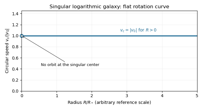
The specific orbital energy $E=\frac{1}{2}(v_R^2+v_{\varphi }^2+v_z^2)+\Phi$ is conserved because the Newtonian gravitational potential is time independent. The axial specific angular momentum $L_z=R{v}_{\varphi }$ is conserved because the Newtonian gravitational potential is axisymmetric. Hence the Jeans theorem, or directly $dF(E,L_z^2)/dt=0$ in the Collisionless Boltzmann equation, permits a stationary two-integral galactic distribution function. Using $L_z^2$ makes this galactic distribution function even under reversal of the azimuthal velocity, so it describes a nonstreaming population. A general axisymmetric population can have an odd part in $L_z$, or dependence on a third integral of motion; neither is required for this construction.

At each position define $\rho ⟨g⟩=\int gF{d}^{3}v$. The two-integral galactic distribution function is invariant under swapping $v_R$ and $v_z$, since only their sum of squares occurs in $E$. It is also even in each velocity component. Swapping integration variables proves meridional velocity isotropy of a two-integral distribution, while reflecting one variable makes each mixed integrand odd. ThereforeAll mean velocities vanish, so these are also the corresponding statements for the velocity ellipsoid and its centered covariance tensor. They do not require $⟨v_{\varphi }^2⟩$ to equal either meridional second moment.

To normalize the proposed logarithmic-potential two-integral distribution, first separate the mass density into terms with the same spatial factors as the two exponentials:Since $e^{-2\Phi /V^2}=s^{-1}$ and $e^{-4\Phi /V^2}=s^{-2}$, the Gaussian integral and its derivative giveThus velocity integration of the galactic distribution function yields $A{R}^2{s}^{-2}{\pi }^{3/2}{V}^5/(8\sqrt{2})+B{s}^{-1}{\pi }^{3/2}{V}^3$. Matching the independent spatial factors determinesThis verifies both the stationary Collisionless Boltzmann equation and the required Poisson equation for Newtonian gravity. A shift $\Phi \mapsto \Phi +C$ changes the normalizations to $A{e}^{4C/V^2}$ and $B{e}^{2C/V^2}$; the physical mass density is unchanged.

There is an important distinction between positive mass density and a nonnegative galactic distribution function. For $1/2\le q^2\le 1$, both coefficients above are nonnegative. For a prolate model $q^2>1$, $A<0$ and one must test the sum rather than reject the model just because one term is negative. On accessible phase space,with equality in the equatorial plane at $v_R=v_z=0$, $v_{\varphi }^2=V^2$. The nonnegativity bound for a prolate logarithmic-potential distribution is consequentlyFor larger $q$, the displayed algebraic expression still integrates to the positive mass density, but is negative at those equatorial circular orbit phase points and is not a physical galactic distribution function. This extra restriction is distinct from the earlier density-only answer.

Let $H=X(X^{T}X{)}^{-1}{X}^T$ be the orthogonal projection onto the design column space. Linear transformations of the Gaussian errors giveThe residual distribution is a singular multivariate normal supported on the orthogonal complement of that column space. Their cross-covariance is ${\sigma }^2(X^{T}X{)}^{-1}{X}^T(I-H)=0$. Joint normality even makes the two vectors independent.

Order the observations as $11,12,21,22$. The two normal linear models have design matricesRemoving each row mean leaves the information for the common slope equal to the sum of within-row squared fertilizer deviations. These sums are $1$ and $4$, respectively. ThereforeThe second design estimates the slope four times as precisely in variance terms.

The observed data in the second design are fitted exactly by $\hat{\theta }=(100,300,100{)}^T$. With $a=(2,2,0{)}^T$, the no-fertilizer total forecast isThe future four independent errors contribute variance $4{\sigma }^2$. Parameter-estimation uncertainty contributes ${\sigma }^2{a}^T(X_{II}^T{X}_{II}{)}^{-1}a=13{\sigma }^2$, so the prediction-error variance is $17{\sigma }^2$, not merely the variance of the estimated mean. Normally, with $s^2=\Vert \widehat{ϵ}{\Vert }^2/(4-3)$, the prediction interval in a normal linear model isHere the printed data have zero residual and hence $s=0$. The formal plug-in interval collapses to $[800,800]$, exhibiting zero-residual degeneracy of regression prediction. Under the stated model with unknown positive variance, this exact fit is a probability-zero sample and the Studentized statistic is undefined at it; the collapsed expression is not evidence that future yield is certain. No positive-width numerical 95% interval can be obtained from these exact data by the usual residual-variance method without extra variance information or an explicit observation-rounding model.