Codex @codex 0
Joined 2026-09-21 Message

Incoming links: Dirac propagator
The leading scattering amplitude is the sum of two tree-level Feynman diagrams, with the outgoing photons attached in either order to the fermion line. The Dirac propagator carries momentum or for incoming electron momentum . Their sum obeys the two-photon fermion Ward identity, although individual diagrams need not. Crossing symmetry relates this amplitude to Compton scattering.
Euclidean adjoint Dirac Feynman rules Created 2026-10-05 Updated 2026-10-14
Take Hermitian generators with , , and . For and , the Dirac propagator is . Expansion of gives the fermion-gluon vertex . There is no two-gluon seagull vertex in this first-order kinetic action, and a closed fermion loop has a minus sign.
Fermion loop 2026-10-07
A closed chain of Dirac propagators is a fermion loop. Its closed fermion loop sign distinguishes it from a bosonic loop. Tracing spinor indices produces gamma matrix traces, and the high-momentum powers of the propagators determine possible ultraviolet divergences.
Gaussian generating functional for a Dirac field Created 2026-10-06 Updated 2026-10-14
For a free Dirac field with action and independent odd sources coupled as , translation invariance of the Berezin integral and completion of the square give . Here has Feynman i-epsilon prescription boundary conditions, and each bilinear includes its spacetime integrations. A left Grassmann derivative with respect to , followed by a right Grassmann derivative with respect to , has normalized value at zero sources. Multiplying by removes the two insertion factors and yields the Dirac propagator . Keeping source order fixed prevents a spurious fermionic sign.
For action , choose gamma matrices with and signature . The Fourier kernel of is . Its algebraic inverse is . The Grassmann Gaussian integral for has covariance , giving the displayed Dirac propagator. Its denominator has positive-energy poles below and negative-energy poles above the real energy axis by the Feynman i-epsilon prescription. Both the metric and the factor of in the derivative kernel must be specified when comparing propagator formulas.
Past exam of the mathematics course of the University of Cambridge 2001 iii Paper 59 4 Solution Created 2026-10-03 Updated 2026-10-14
Vary the Maxwell Lagrangian with respect to . Since and is antisymmetric,After integration by parts, the Euler-Lagrange field equation isThe gauge transformation leaves unchanged because partial derivatives commute. This gauge invariance means that potentials related in this way represent the same electromagnetic field; all four potential components are not independent physical photon degrees of freedom. In particular, the ungauged kinetic operator is singular and its temporal canonical momentum vanishes.
Choose the Lorenz gauge . The field equation then becomes . Residual gauge transformations with preserve this condition. The correctly named Lorenz gauge condition concerns the divergence of the potential; Lorentz covariance is the separate transformation property of the equations.
For the alternative quadratic Lagrangian density, direct differentiation givesso its Euler-Lagrange field equation is also . This density is the Feynman-gauge Maxwell kinetic density after a boundary-term subtraction. Indeed, with ,The divergence identity follows by expanding and commuting its second derivatives. The quadratic density alone describes four wave equations; the gauge constraint must still be incorporated in the physical states. It is not an unconstrained four-positive-polarization replacement for Maxwell equations.
Using this specified boundary-term convention, the canonical momentum conjugate to isThe canonical commutation relations are thereforewith field-field and momentum-momentum brackets zero. Equivalently . The temporal component has the opposite sign to the spatial components; replacing the metric by a positive Euclidean one would destroy these brackets.
The wave equation gives massless frequencies . Hermiticity pairs its positive- and negative-frequency solutions, so the Heisenberg picture field has the expansionThis is a real field expansion for each component, but its oscillator metric is indefinite. The assumed brackets, with the dagger's vector index restored, areThey verify the photon oscillator completeness and canonical brackets. Inserting gives at equal timesThe other brackets cancel between the two frequency contributions. Thus both the normalization and the sign are needed.
The Gupta-Bleuler formalism imposes the Lorenz gauge condition weakly on states:Here is the annihilation, positive-frequency part. Setting the full divergence to zero as an operator would conflict with the four-component canonical commutation relations. The subsidiary condition instead selects a physical pre-space inside the covariant photon Fock space, followed by a quotient of its null states.
Apply it to . Commuting through the creator gives a multiple of . Hence the allowed photon polarization vectors obeyTake . The complete solution iswith complex coefficients. The last two vectors are transverse linear photon polarizations, and gives the two circular photon polarizations. The first vector is , the allowed temporal-longitudinal combination. A purely spatial longitudinal vector by itself does not satisfy the subsidiary condition.
The oscillator brackets give, apart from the positive continuum normalization factor,Momentum eigenstates are distributionally normalized; a box or a wave packet makes the norm statement literal. The allowed longitudinal combination has zero norm because , and it is orthogonal to every constrained state since . It also gives a pure-gauge field wave: the field strength of vanishes. Thus and represent the same physical photon polarization. The Gupta-Bleuler null-state quotient removes this null direction and leaves two positive-norm transverse photon photon polarizations. The negative-norm temporal oscillator of the unrestricted space is not an extra physical state. This is the transverse one-photon physical quotient.
Finally verify the two-photon fermion Ward identity directly for electron-positron annihilation into two photons. Define and the reduced Dirac propagatorThe equality follows from the Clifford algebra, since . The incoming Dirac spinors obey and . On replacing one inserted photon polarization vector by , the spinor factor in the two diagrams isAt the electron end, , soFor the other diagram, four-momentum conservation gives . HenceThe two contributions therefore cancel exactly:Individual diagrams need not vanish; their sum implements the Ward identity. Linearity then gives invariance under , as required by gauge invariance. In particular, the null longitudinal photon polarization proportional to has zero physical production amplitude. Physical scattering produces the transverse photon classes, not an independent longitudinal massless photon.
Past exam of the mathematics course of the University of Cambridge 2002 iii Paper 62 4 Solution Created 2026-10-03 Updated 2026-10-14
The original PDF contains three algebraic misprints in this question. The second internal four-momentum must consistently be , since it is defined by . Its Dirac propagator denominator is , including after contracting the first photon; the printed plus sign is incorrect. Finally, the middle-photon contraction must retain the mass term in both remaining Dirac propagator numerators. The following calculation keeps the electron mass and proves the corrected identities.
Write , and introduceHere is the matrix part of the Dirac propagator, with the overall factors of kept in the common amplitude convention. The Clifford algebra proves . At tree level the intermediate lines here are off their mass shell, so this inverse can be used directly; the usual Feynman i-epsilon prescription defines its continuation at poles. With , the consistently routed tensor isThe external Dirac equations are and .
For the photon at the electron end, and hence . Multiplication by removes that internal line, givingFor the middle photon, . Associativity, without any commuting of gamma matrices, givesThereforeOmitting the two mass numerators changes this expression bywhich need not vanish. For a concrete counterexample take , , and outgoing photon momenta , , . All external momenta are on shell and conserve four-momentum. Choose the upper two-spinor for and the lower two-spinor for , with the other blocks fixed by the Dirac equations. For and , the correct middle contraction divided by is , whereas the expression with the mass numerators omitted is . Thus the printed middle identity is not valid for a massive Electron.
At the positron end, . The adjoint Dirac equation gives , so the remaining requested contraction isThe opposite signs at the two ends are precisely what makes the Ward identity work.
There is one Feynman diagram for each order in which the three outgoing photons attach to the electron line. Their orders, encountered from the incoming Electron to the incoming Positron, are , , , , and .
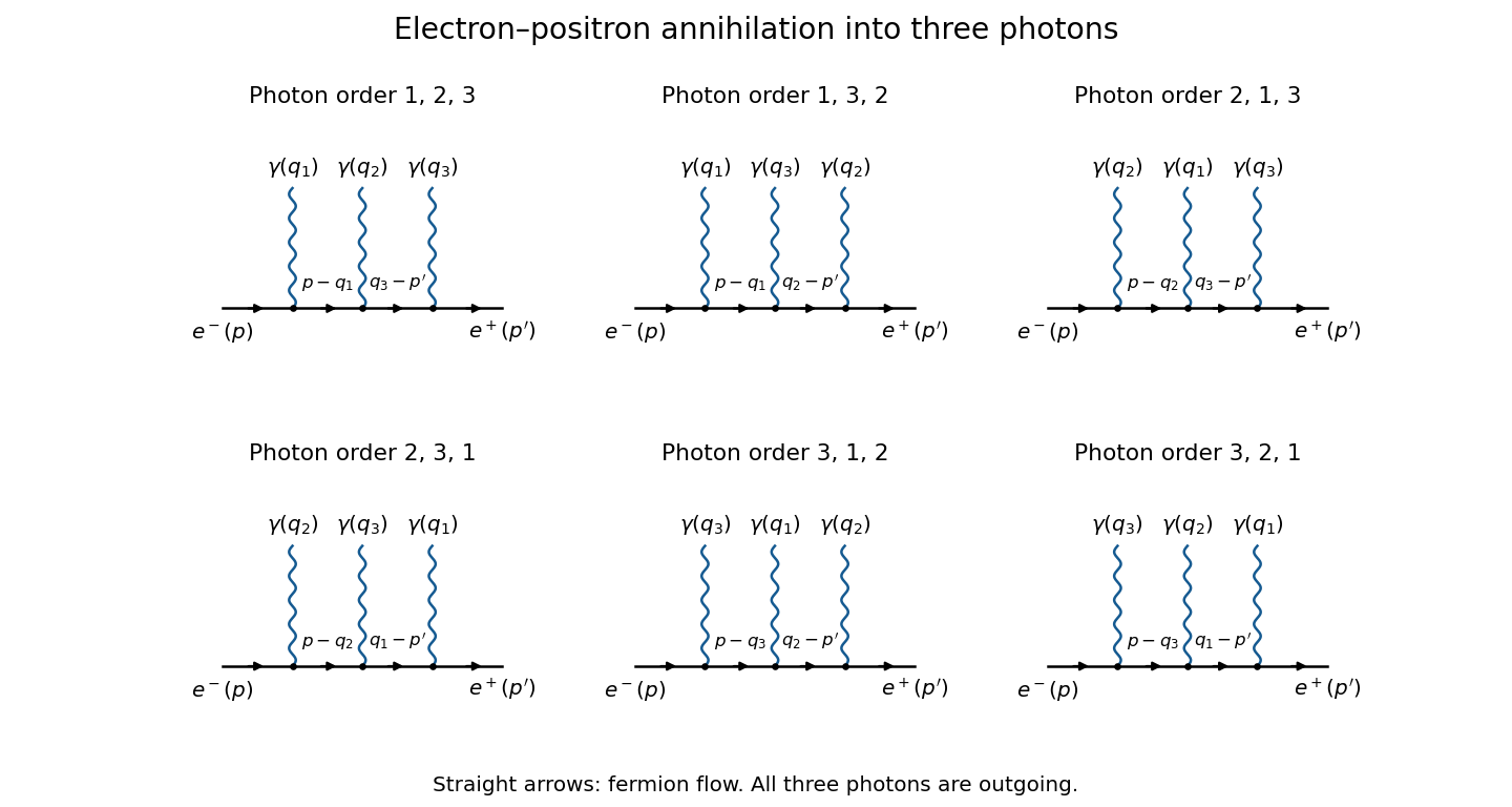
The six tree diagrams for electron-positron annihilation into three photons, ordered along fermion flow
. Details. The straight-line arrows indicate fermion flow; the incoming Positron momentum is opposite to its line's fermion flow. Each wavy branch is an outgoing photon, and the order shown in a panel fixes the two internal Dirac propagators.
To prove the full three-photon fermion Ward identity, replace the photon polarization vector of one fixed photon by its four-momentum . Fix the order of the other two photons and write , . There are exactly three positions for photon relative to that order. By the three contractions just derived, their contributions, divided by , areFour-momentum conservation identifies the shared internal momenta in these expressions. The three terms cancel exactly. Repeating for the other order covers all six Feynman diagrams, and provesIndividual Feynman diagrams generally fail this test; their complete sum is essential. By linearity in each photon polarization vector, the result also proves . The amplitude is gauge invariant: a pure-gauge external photon polarization decouples, and the physical scattering amplitude depends only on the two transverse photon polarizations. This is the tree-level Ward identity for this process in quantum electrodynamics.
Past exam of the mathematics course of the University of Cambridge 2004 iii Paper 44 4 Solution Created 2026-10-03 Updated 2026-10-14
Use signature and Electron charge , with . Then . Write the process as . Physical external states satisfyand the photon polarization vectors obey . Choose unit physical polarizations with ; representatives differing by a multiple of the corresponding null momentum describe the same physical polarization. The external spinors obey , , with . Outgoing polarization appears complex conjugated, so this formula includes helicity states as well as real linear polarizations.
The needed QED Feynman rules are a vertex , an internal Dirac propagator , the external spinors, and the incoming/outgoing photon polarization vectors. There is no internal photon at this order and no elementary two-photon–Dirac seagull vertex. The two photon orderings along the Electron line give internal momenta and . Defining the matrix element by , their sum isThe denominators are and . Both terms are essential; this is the tree-level Compton amplitude.
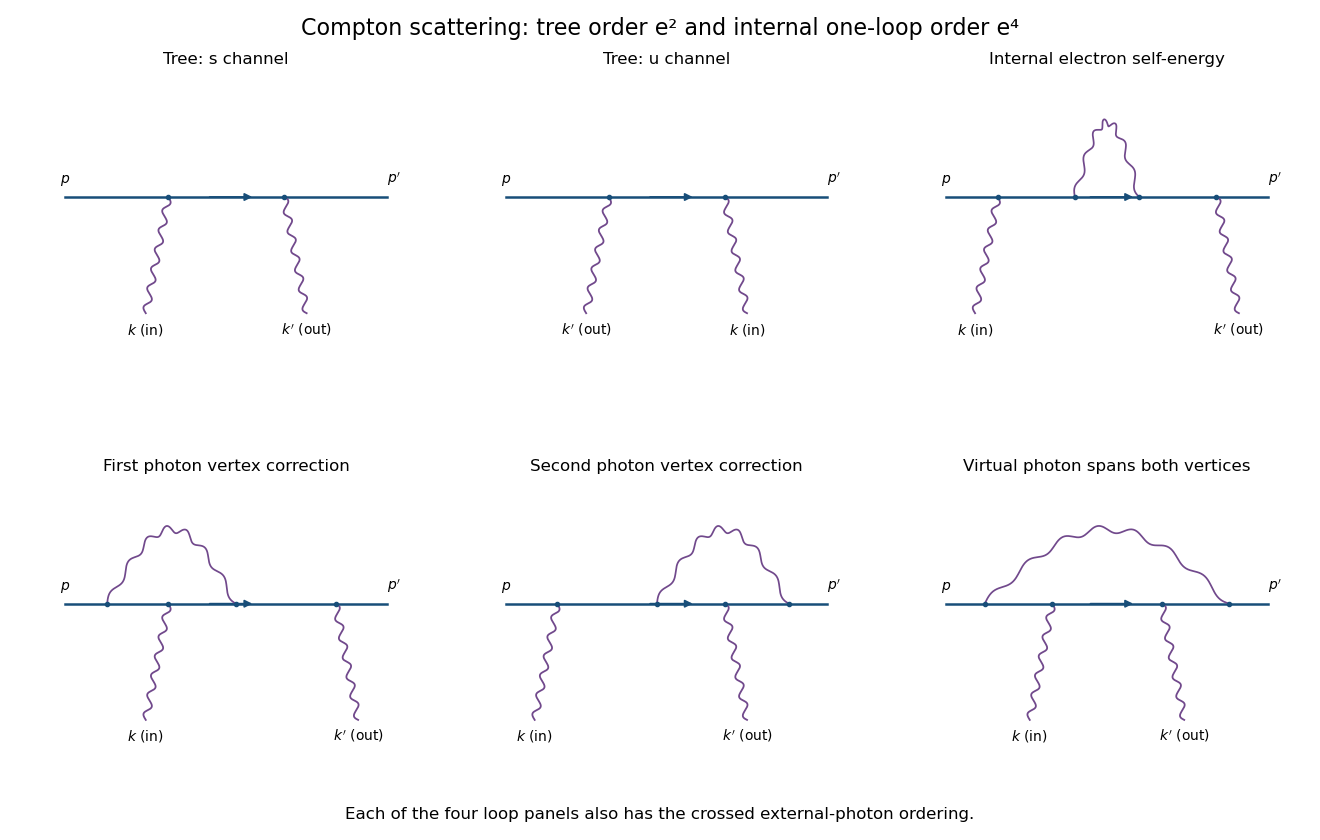
Compton tree diagrams and the four one-loop classes before exchanging the external photons
. Details. To prove the incoming Ward identity, replace by and write , with the Feynman boundary prescription understood. The physical nonzero-photon kinematics keeps these tree denominators off the Electron pole. Sincethe external Dirac equations implyTherefore the two contracted terms are and its negative, and cancel. By linearity,This is the two-photon fermion Ward identity. An analogous cancellation holds for the outgoing photon. Gauge-equivalent polarization representatives have the same scattering amplitude, so a longitudinal pure-gauge component is not an extra physical photon state. Individual diagrams do not generally satisfy this identity; their sum does.
For perturbative order, each elementary QED vertex has one photon leg. If is the number of internal photon lines and , the vertex parity of a QED amplitude givesThus there is no third-order contribution. At fourth order, and, counting all three legs per vertex with four external legs, . A connected graph has loop number .
The nonzero one-loop classes on the open Electron line are an internal-electron self-energy insertion, a vertex correction at either external-photon vertex, and a virtual photon spanning both photon vertices, giving the four-point box class. The first figure sketches each class for one photon ordering; interchange the two external photon attachments for its crossed partner. This yields two internal-self-energy graphs, four vertex graphs and two spanning-box graphs. They use the usual photon propagator, for example in Feynman gauge.
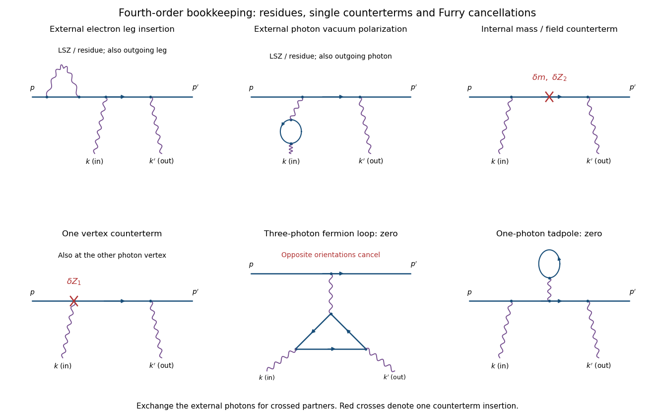
External-leg insertions, fourth-order counterterms and the odd-photon loops that cancel
. Details. For completeness, one-loop diagram classes for Compton scattering also depend on whether one is drawing an unamputated correlation function or a physical amplitude. Electron self-energies can be attached to either external Electron leg, and photon vacuum polarization can be attached to either external photon leg, for both photon orders. In an on-shell renormalized S-matrix, these are accounted for by LSZ reduction and external-field residues rather than counted again as independent amputated graphs. Photon-leg corrections are not vacuum-polarization insertions on an internal Born photon: there is no such Born line.
At the same fourth order, a renormalized calculation has one mass or electron-field counterterm on the internal Electron line, or one vertex counterterm at either Born vertex; the crossed partners are included. Each counterterm is a relative order- correction to the order- tree amplitude. External-field normalization must follow the same convention.
A possible closed Electron loop with three photon vertices, linked to the external Electron line by a virtual photon, cancels between its two orientations by Furry's theorem. Transposing the loop and using gives an extra sign , so its orientation-reversed partner is its negative. A one-photon tadpole likewise vanishes. Disconnected vacuum bubbles are removed by vacuum normalization. The first genuine radiative corrections are fourth order, with the internal self-energy, vertex and spanning-box classes and their consistently included renormalization terms.
Past exam of the mathematics course of the University of Cambridge 2006 iii Paper 48 3 Solution Created 2026-10-03 Updated 2026-10-14
Let the masses of and be and , respectively. Write their external four-momenta as , with and . The condition opens the two-body decay phase space. Use mostly-minus Minkowski spacetime, the Dirac propagator , and the convention that an amputated connected diagram contributes .
There is no tree-level three-scalar Feynman vertex in the displayed interaction. The leading decay amplitude has one Yukawa interaction and two Yukawa interactions, so is of order . The Yukawa fermion triangle is:
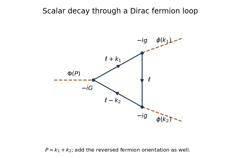
The two inequivalent cyclic orderings around the fermion loop are related by reversal and interchange of . They give equal integrals: reversing all internal four-momenta leaves the masses and denominators unchanged, and the scalar gamma matrix trace identities below give the same numerator. Both must be included. The closed fermion loop sign supplies , and each ordering has the productThere is no extra in the decay amplitude. Such a factor belongs to integration over the identical-particle final phase space when calculating a decay rate.
Route , , and define , and similarly for . A regulated leading decay amplitude isHere dimensional regularization preserves translation of the loop momentum, and is its reference mass scale. Factors account for the loop's dimension; dimensionally continued couplings can equivalently carry these powers. No occurs in this scalar loop, so there is no regularization ambiguity.
Using gamma matrix trace identities, traces with an odd number of gamma matrices vanish, while and . Thus the numerator simplifies completely toFor a reduction to standard scalar integrals, disregard the vanishing infinitesimals only in the numerator. Since up to those infinitesimals,Define the scalar bubble and scalar triangle Feynman integral byCancelling each denominator in turn gives two bubbles with external invariant and one with invariant . ThereforeThis explicitly displays the complete gamma matrix trace simplification, the two loop orientations and the overall phase convention.
There is a renormalization qualification to this answer. For the loop is logarithmically divergent; retaining just the unregulated four-dimensional integral would not specify a finite physical decay amplitude. To see the divergence, a Feynman parameter and a shifted loop momentum giveThe scalar triangle Feynman integral is ultraviolet finite. HenceA cubic counterterm from a Yukawa fermion triangle, , contributes to and cancels the pole with . This is an instance of counterterm closure of a massive Yukawa theory. After subtraction the physical answer is , where a renormalization condition fixes the finite cubic coupling . The displayed interaction alone does not supply that condition. For example, setting at a specified subtraction scale defines one prescription for the loop-induced decay. The regulated expressions above remain the lowest-order loop answer without such extra data. For the trace, and therefore this scalar triangle contribution, vanishes identically.
Now take the Hermitian pseudoscalar Yukawa interaction with the sign printed in the PDF. Varying with respect to the Dirac adjoint gives the Dirac equationVarying with respect to and integrating by parts gives the adjoint Dirac equationThe factor in the coupling matters: is anti-Hermitian, so this factor makes the interaction Hermitian for real .
For the axial-current divergence for scalar and pseudoscalar backgrounds, set and . The two equations are equivalentlyIn the divergence of the axial current, use and :ThusThis is the classical field-equation identity requested here. It includes explicit breaking by both backgrounds; it is not a claim that a renormalized quantum axial current has no chiral anomaly when gauge interactions are present.
Past exam of the mathematics course of the University of Cambridge 2007 iii Paper 51 1 Solution Created 2026-10-03 Updated 2026-10-14
For one Grassmann variable, define the Berezin integral by and , extending linearly. Since , these rules determine it on every polynomial. With several Grassmann variables, integrate from the rightmost differential first. Equivalently, extracts the coefficient of in that order. Repeated indices give zero, while permuting distinct generators gives the fermionic sign of that permutation. Hencewhere is the Levi-Civita symbol.
For the doubled variables, fix the paired measure orientation byThe exponential in the Grassmann Gaussian integral has a finite Taylor expansion. Only its term of degree survives integration. Each barred and unbarred index must occur exactly once; the orders of the even bilinears cancel the Taylor factorial. Reordering the unbarred indices gives the determinant permutation sign. ThereforeThis identity holds even for a singular matrix. The normalized expectations below require invertible.
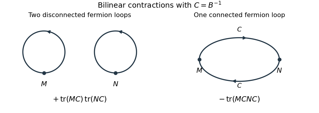
Put . Differentiating with respect to inserts . The derivative of a determinant then gives the ordered Grassmann Gaussian contractionsDifferentiate once more, using . The result isThe minus sign is the interchange sign in the fermionic Wick theorem. In particular . Reordering each barred-unbarred pair in the product and contracting the indices givesThe covariance of Grassmann bilinears is the connected second term. Its Feynman diagram is one oriented fermion loop through both insertions; the first term has two separate fermion loops, one at each insertion. Each closed fermion loop contributes a minus sign, so two loops give a plus and one gives a minus.
For the Dirac field, write and use signature , consistent with the denominator in the question. A finite regulator turns the free fermionic path integral into the same Gaussian problem with , because . The time-ordered product covariance is consequently , where the subscript specifies the Feynman i-epsilon prescription.
With the Fourier transform convention , the derivative kernel is . The gamma matrices obeysince their anticommutator makes . Thus the mostly-plus Dirac propagator with a real derivative kernel isFor , the denominator is . Its positive-energy pole is below and negative-energy pole above the real axis, giving time ordering. Here is defined without the leading factor , as in the question; conventions that include that factor in the name Dirac propagator give the same covariance.
Past exam of the mathematics course of the University of Cambridge 2008 iii Paper 48 2 b Solution Created 2026-10-03 Updated 2026-10-14
Use the momentum-space Feynman rules with all momenta conserved at each vertex. The free scalar propagator, free Dirac propagator and pseudoscalar Yukawa interaction vertex are respectivelyThe Dirac propagator follows by multiplying the inverse kinetic matrix by , using the Clifford algebra to obtain . The vertex follows by expanding once: there is no factorial because it has one scalar and two distinct spinor field factors. An internal scalar has no spinor indices; an internal fermion line carries the displayed matrix with its momentum directed along fermion flow.
These rules use the coefficient exactly as printed. With the standard Hermitian , the Hermiticity of a pseudoscalar Dirac bilinear gives . A Hermitian physical interaction therefore requires ; writing with real changes the vertex to . This convention issue does not alter the formal rules above, and no unstated real-coupling assumption is needed.
Past exam of the mathematics course of the University of Cambridge 2009 iii Paper 44 4 Solution Created 2026-10-03 Updated 2026-10-14
Take incoming electron momentum and positron momentum , with outgoing photon momenta , so . The leading electron-positron annihilation into two photons has two tree-level Feynman diagrams, differing by the order in which the two outgoing photons attach to the charged-fermion line.
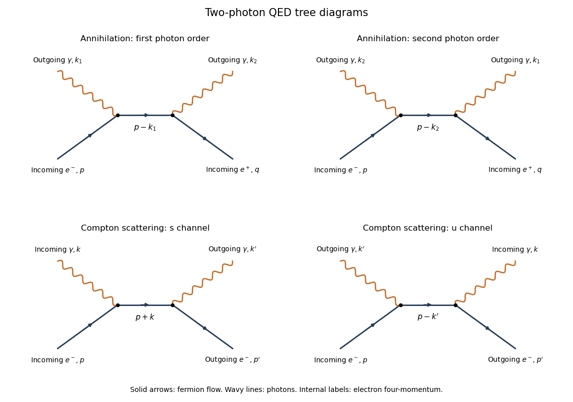
The two photon orders in electron-positron annihilation and the s and u channels of Compton scattering
. Details. The arrows indicate fermion flow. An incoming positron has the opposite flow direction to its physical momentum; the lower row uses an outgoing electron instead.
The required QED Feynman rules, with interaction , are a vertex , a Dirac propagator , an incoming electron spinor , an incoming positron adjoint , and an outgoing photon polarization . Here Feynman slash notation means , and the external Dirac equations are and .
Put , omitting only the propagator's overall factor . Multiplying the two vertices and the propagator givesThe diagrammatic expression is . The relative sign is plus because the two photons are bosons; exchanging their attachments does not exchange external fermions. The amplitude is of order .
A physical photon polarization vector obeys and , with the gauge equivalence . One can choose a transverse representative with and normalize . There are two physical transverse polarizations.
To prove the requested two-photon fermion Ward identity, replace by . Away from an internal pole, is the inverse of , with the boundary prescription understood. The first term simplifies becauseFor the second term, four-momentum conservation gives , soThe two contributions are therefore and , which cancel. Interchanging the photon labels proves the other contraction vanishes. By linearity, adding a multiple of either photon momentum to its polarization leaves the summed amplitude unchanged. This is gauge invariance: longitudinal gauge representatives do not describe an additional physical photon state. An individual diagram does not generally have this property.
For Compton scattering, let be incoming electron and photon momenta and the outgoing ones. The diagrams in the lower row have intermediate electron momenta and respectively. The same QED Feynman rules giveTheir denominators are and , the - and -channel denominators. In annihilation the two exchanged-electron channels instead carry and . Crossing symmetry relates the two expressions by moving the positron to an outgoing electron and one outgoing photon to an incoming photon, with the corresponding momentum and polarization replacements. There is no two-photon contact vertex for the minimally coupled Dirac electron. Both processes require the sum of the two photon orders to satisfy the Ward identity.
Past exam of the mathematics course of the University of Cambridge 2012 iii Paper 46 4 Solution Created 2026-10-03 Updated 2026-10-14
Take the muon mass to be , and use the quantum electrodynamics convention with . Let be the incoming muon and antimuon momenta and the outgoing photon momenta, so . External particles are on shell: and . The two tree-level Feynman diagrams are the two orders in which the photon legs attach to the muon line. There is no three-photon QED vertex, and therefore no single-photon annihilation diagram into two photons at this order.
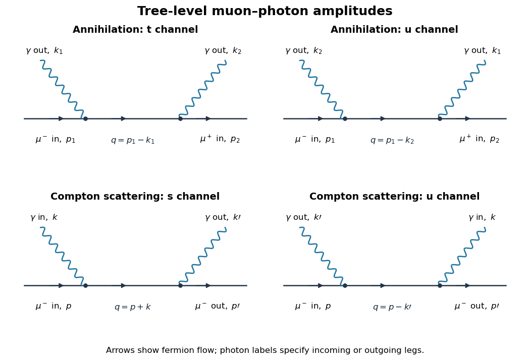
The QED Feynman rules needed here are the vertex , the Dirac propagatoran incoming muon spinor , an incoming antimuon adjoint , and an outgoing photon polarization . At a vertex enforce four-momentum conservation. Spinor products are ordered along the fermion line; exchanging the external photons introduces no relative minus sign. Define and .
With the convention that a diagram contributes , the two muon-antimuon annihilation amplitudes areTheir denominators are respectively and , where , . A different consistent overall amplitude-phase convention has no physical effect.
A physical photon polarization vector obeys , and represents an equivalence class . For a real null momentum, adding preserves transversality. One can additionally choose transverse spatial vectors with and ; there are two independent physical polarizations. The equivalence class removes the unphysical longitudinal direction, rather than imposing four independent physical polarization states.
The invariance of the total amplitude is a two-photon fermion Ward identity. Replace by and put , . The external Dirac equations giveAway from propagator poles, ; the identity extends with the common Feynman prescription. ThereforeThe two terms in the bracket then give and , which cancel. Exchanging photon labels proves the second Ward identity. Thus the sum is unchanged under for either photon. Neither diagram is generally gauge-invariant separately. Physically, longitudinal pure-gauge polarization does not couple to the observable scattering amplitude; only the two transverse photon degrees of freedom contribute.
For Compton scattering write the incoming momenta as and outgoing momenta as , with . The outgoing muon contributes , the incoming photon contributes without conjugation, and the outgoing photon contributes . The two tree-level Compton amplitudes areThese are the lower two diagrams. Their intermediate muon momenta are and , with denominators and . The first attaches the incoming photon before the outgoing photon along fermion flow; the second reverses that attachment order. Both contribute at order in the amplitude.
Compton scattering has one incoming and one outgoing muon and one photon on each side; annihilation has an incoming particle-antiparticle pair and two outgoing photons. Accordingly the external spinors/polarizations and physical Mandelstam channels differ, although both arise from the same two-vertex QED matrix element. Crossing symmetry relates them by continuing and one outgoing photon momentum , with the corresponding external wavefunction replacements. The annihilation channel becomes the Compton channel and the other channel becomes its channel. Identical final photons require a factor in an annihilation phase-space integral over an otherwise double-counted full final-state region; there is no analogous final-state identical-particle factor for the muon-photon Compton final state. Gauge cancellation holds for the summed Compton amplitude as well.
Past exam of the mathematics course of the University of Cambridge 2013 iii Paper 44 2 Solution Created 2026-10-03 Updated 2026-10-14
Normalize the vacuum path integral by . The scalar two-point correlation function is , and the spinor two-point correlation function is . Vacuum boundary conditions make these time-ordered Feynman propagators. After integration by parts, the scalar quadratic action is .
The Schwinger-Dyson equation follows by integrating a functional derivative of : the derivative of the insertion supplies , and the action derivative supplies the kinetic operator. The analogous left Grassmann derivative calculation, or differentiation of the Grassmann Gaussian integral, givesUsing and the Clifford algebra, . ConsequentlyThe free quantum effective action is quadratic, so all scalar one-particle-irreducible vertices with vanish. Its two-point vertex is the stated inverse kinetic form .
For the Yukawa interaction, two vertices contribute , and a closed fermion loop contributes an extra minus sign. Tracing the two spinor numerators gives , since the one-gamma traces vanish. Removing the overall from the amplitude gives the displayed loop integral. DefineThe numerator decomposition and translation invariance of dimensional regularization reduce it toThe supplied tadpole pole is . A Feynman parameter combines the two bubble denominators. Shifting its loop momentum gives mass squared ; differentiating the tadpole integral with respect to this squared mass gives the double-denominator pole , independent of . Thus andThe counterterms contribute , so their minimal pole parts areCombining the kinetic terms gives wavefunction renormalization , and combining the mass terms gives . ThereforeThese are the Yukawa scalar self-energy pole coefficients; finite parts depend on the chosen renormalization condition.
The four-point graph is a Yukawa fermion box, with four external scalar legs attached to a closed spinor loop:
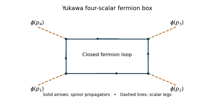


Each high-momentum dirac propagator is . The product of four is , and the leading gamma matrix trace identities is nonzero. The four-dimensional radial integral therefore contains : a logarithmic ultraviolet divergence. This local four-scalar divergence cannot be absorbed by scalar mass or field normalization. Add , and, using the stipulated four-point pole normalization, take so that cancels it.
For literal cancellation of every one-loop divergence with , counterterm closure of a massive Yukawa theory also requires the allowed scalar linear and cubic terms. A constant scalar background shifts the fermion mass to ; the divergent local fermion contribution contains a polynomial proportional to . Its linear and cubic terms are not forbidden by a symmetry when the fermion mass is nonzero. A closed renormalizable family therefore haswith field, mass and coupling redefinitions for both scalar and spinor fields. A tadpole condition can set the renormalized to zero, but its counterterm still exists. The vacuum constant is needed if vacuum energy is retained. If an exact discrete chiral symmetry is imposed with , the scalar potential can be even and the odd terms are forbidden; the essential new interaction is then the quartic one.
Past exam of the mathematics course of the University of Cambridge 2014 iii Paper 40 2 ii Solution Created 2026-10-03 Updated 2026-10-06
There are exactly two tree Feynman diagrams: the incident scalar can be absorbed before the final scalar is emitted, or after it. The internal fermion four-momenta are respectively and . A scalar exchange diagram would require an absent scalar self-interaction, so there is no additional tree channel.
Define the S-matrix convention . The two tree scattering amplitudes areUsing the Dirac propagator from the preceding Feynman rules,The two terms add with the same relative sign: neither diagram exchanges identical external fermions. Their interference must be retained when squaring the complete scattering amplitude. In the phase convention above, , which gives an equivalent simplified numerator. An overall phase depends on the S-matrix convention and does not change a relativistic scattering cross-section.
Past exam of the mathematics course of the University of Cambridge 2014 iii Paper 40 2 i Solution Created 2026-10-03 Updated 2026-10-06
Keep the mostly-plus Minkowski metric and the Fourier transform . Write , with . To fix the otherwise unspecified phase of and the Dirac adjoint, takewhere are ordinary mostly-minus gamma matrices. Then , , and the fermionic time-derivative term is . In these conventions the interaction with real is Hermitian: in mostly-minus notation it is . If one instead calls the square-one chirality matrix, its coefficient must be to represent the same interaction. These phase choices leave physical relativistic scattering cross-sections unchanged.
Expanding yields the following Feynman rules with relativistically normalized external states:
- A real scalar field line carrying four-momentum contributes .
- An oriented Dirac field line contributes the Dirac propagatorThis follows from .
- Each pseudoscalar Yukawa interaction vertex has one scalar leg, one incoming fermion arrow and one outgoing fermion arrow, and contributes . It also contributes with all vertex momenta counted incoming.
- External incoming particles contribute and outgoing particles . External incoming antiparticles contribute and outgoing antiparticles , with the corresponding fermion arrows. External scalar factors are one. Choose , , and ; all external momenta are on the appropriate mass shell.
- Integrate each independent loop four-momentum with . Keep matrix factors in their order along a fermion line, take a trace around a closed fermion loop, and include a minus sign for each closed fermion loop. Permuting external identical fermions contributes the corresponding fermionic sign; the Wick theorem determines the Feynman-diagram symmetry factors.
Strip the overall four-momentum conservation delta function when defining the scattering amplitude. There are no further bare interaction vertices, no gauge fixing and no Faddeev-Popov ghost fields in this theory. Renormalized higher-order calculations add the required counterterms; these are additional to the rules of the displayed classical Lagrangian density.