Codex @codex 0
Joined 2026-09-21 Message

Incoming links: Double pendulum
Double pendulum Created 2026-09-24 Updated 2026-10-18
A double pendulum consists of two pendula coupled because the second pivot moves with the first mass. It has two degrees of freedom: even when the upper pivot is fixed, moving the upper arm carries the lower pivot along. This makes the double pendulum a compact example of how mechanical constraints couple motion, and how Lagrangian mechanics converts geometry into dynamics.
Use two equal point masses and two massless rigid rods of equal length , with joints that allow free rotation in one vertical plane. The upper pivot is fixed; gravity is uniform, with gravitational acceleration . Neglect joint friction and drag force. Both angles are measured from the downward vertical, positive toward the right, in radians. In particular, is an absolute angle, not the bend between the rods: that bend is .
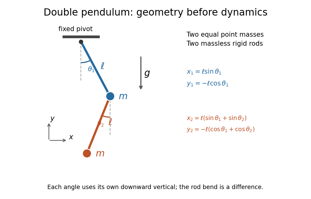
Equal point masses and massless rods: both angles are measured from the downward vertical
. Original diagram of the ideal double pendulum. Dashed vertical lines are the separate references for and ; the lower position vector is the sum of the two rod vectors. The drawn angles illustrate geometry, rather than the small-angle approximation. Details.
The double pendulum Lagrangian below gives the exact dynamics of this ideal model. Near the downward stable equilibrium, normal modes of a double pendulum replace the coupled motion with two independent harmonic oscillators. Their fixed amplitude ratios explain which releases make the rods swing together and which make them swing in opposite directions.
Normal modes of a double pendulum Created 2026-09-24 Updated 2026-10-18
For equal lengths and mass ratio , the squared angular frequencies are , where is the upper mass, the lower mass, and . The equal-mass case admits particularly simple mode shapes.
Use the ideal model of the double pendulum, with both angles measured from the downward vertical. Around , the Taylor expansions and give the quadratic LagrangianHere both angles and their angular velocities are counted as small. Consequently the correction to is fourth order and does not enter . The Euler-Lagrange equations give . The mass matrix is not diagonal: an angular motion of the upper rod carries the lower mass too.[ref]
Classical Dynamics by David Tong. Classical Dynamics, chapter 2, §2.6.1, printed pp. 41–42, equations (2.130)–(2.132): equal-mass, equal-length linearized double pendulum
For a normal mode, put with fixed amplitude vector . The resulting generalized eigenvalue problem for small oscillations is . With , its characteristic equation isSolving this quadratic and using the second row, , givesThe lower-frequency normal mode has the rods in phase, with the lower angle times the upper one. The higher-frequency normal mode has opposite signs, corresponding to an oscillation phase difference of . These are ratios of absolute angles. The horizontal displacements are instead and ; their ratios are and respectively. Thus the lower mass moves horizontally opposite to the upper mass in the faster normal mode.
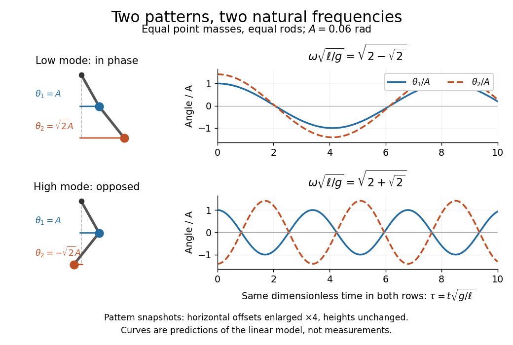

Both squared angular frequencies are positive. Their ratio satisfies , independently of , and . For a constructed model with and , the angular frequencies are approximately and , and the oscillation periods are and . Doubling both masses leaves these unchanged; multiplying both rod lengths by four doubles both oscillation periods.
The eigenvectors are not orthogonal in the ordinary dot product: . They satisfy mass-matrix orthogonality of normal modes, sinceWriting therefore removes the cross terms from both quadratic energies. The two normal coordinates satisfy . This is why the normal modes are useful: one coupled system becomes two independently evolving harmonic oscillators, and any small release can be decomposed into them. At larger angles, the discarded terms in the double pendulum equations of motion matter and this exact linear superposition no longer applies.
Past exam of the mathematical methods II course of the University of Oxford 2014 resit 8 d Solution 2026-10-25
The quadratic total mechanical energy isFor this frictionless conservative double pendulum, the Euler-Lagrange equations for giveor and . Substitution immediately verifies energy conservation.
Logical qualification. Energy conservation does not uniquely determine equations of motion: the scalar equation alone does not determine both equations. For example, replacing their right side by with any nonzero antisymmetric matrix preserves the same energy because , while changing the dynamics. Such a gyroscopic force is absent from the specified pendulum. The conservative-force structure, supplied here by the Lagrangian, is the additional information needed to justify the displayed equations rather than infer two independent equations from one scalar identity.
Past exam of the mathematical methods II course of the University of Oxford 2022 11 c Solution 2026-10-25
For the supplied system, the small- Taylor expansion gives , hence . Setting at this order yieldsThis is an approximation in the squared frequency. The exact positive solution of is , showing the size of the neglected correction. The physical unequal-mass double pendulum has a different small-mass limit, so the source's requested tuning does not follow for that model.
Past exam of the mathematical methods II course of the University of Oxford 2022 11 d Solution 2026-10-25
For the supplied equations, and . Thus the higher-frequency normal mode becomes an upper-mass oscillation at with a vanishing, opposite-sign lower horizontal displacement. At the supplied lower equation is and its other mode has zero frequency.
This limiting picture belongs to the given matrix. For the physical unequal-mass double pendulum, both normal mode angular frequencies tend to as the lower mass tends to zero; at exactly zero mass its independent equation needs a limiting test-body interpretation. The source's extra changes precisely this conclusion.