A double pendulum consists of two pendula coupled because the second pivot moves with the first mass. It has two degrees of freedom: even when the upper pivot is fixed, moving the upper arm carries the lower pivot along. This makes the double pendulum a compact example of how mechanical constraints couple motion, and how Lagrangian mechanics converts geometry into dynamics.
Use two equal point masses and two massless rigid rods of equal length , with joints that allow free rotation in one vertical plane. The upper pivot is fixed; gravity is uniform, with gravitational acceleration . Neglect joint friction and drag force. Both angles are measured from the downward vertical, positive toward the right, in radians. In particular, is an absolute angle, not the bend between the rods: that bend is .
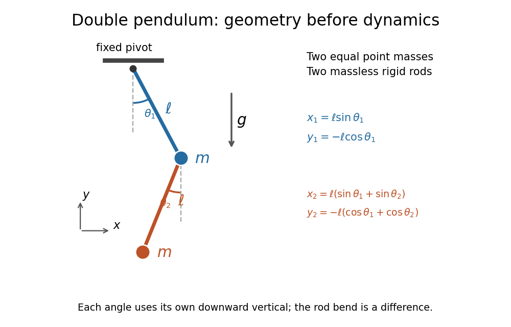
Equal point masses and massless rods: both angles are measured from the downward vertical
. Original diagram of the ideal double pendulum. Dashed vertical lines are the separate references for and ; the lower position vector is the sum of the two rod vectors. The drawn angles illustrate geometry, rather than the small-angle approximation. Details.The double pendulum Lagrangian below gives the exact dynamics of this ideal model. Near the downward stable equilibrium, normal modes of a double pendulum replace the coupled motion with two independent harmonic oscillators. Their fixed amplitude ratios explain which releases make the rods swing together and which make them swing in opposite directions.
With equal rod lengths and absolute downward-vertical angles , the endpoint separation is . A zero-rest-length spring between the fixed support and the final mass contributes to the Lagrangian. It favours bending away from maximum extension and can reduce the gravitational bending stiffness.
Choose Cartesian coordinates with origin at the upper pivot, to the right and upward. The two position vectors areThese expressions satisfy the rod holonomic constraints and automatically. This is the practical advantage of using the two angles as coordinates: the rod tensions need not be unknowns in the motion calculation.[ref]
Classical Dynamics by David Tong. Classical Dynamics, chapter 2, §2.3, printed pp. 17–19: elimination of ideal constraint forces using coordinates adapted to holonomic constraints
Differentiate these position vectors to obtain the velocities. The dot product between their two rod contributions uses , givingAdding the two kinetic energies and measuring gravitational potential energy from the downward equilibrium givesThe coefficient has a geometric meaning: the upper rod raises both masses, and its motion contributes to both kinetic energies. The coupling in is present because the lower mass has a moving pivot. The zero chosen for changes by a constant and leaves the Euler-Lagrange equations unchanged.[ref]
Classical Dynamics by David Tong. Classical Dynamics, chapter 2, §2.5.2, printed p. 28, equations (2.68)–(2.72): general point-mass double pendulum; the derivation here specializes to equal masses and lengths and uses upward
The principle of stationary action applies to . Its fixed-endpoint first variation, after integration by parts, isIndependent allowed variations therefore give one Euler-Lagrange equation for each angle. Stationary action alone does not assert a minimum.[ref]
Write . Applying the Euler-Lagrange equations to the double pendulum Lagrangian, then dividing by , givesFor example, the upper generalized momentum is . Its time derivative contains . Subtracting cancels the mixed product and leaves the positive term in the first equation. This cancellation is a useful check on the sign convention.
The matrix multiplying the two angular accelerations isIt is invertible for every configuration, so specified angles and angular velocities determine both angular accelerations. For the same reason whenever the angular velocities are not both zero. The mass cancels from the motion equations, while the timescale is set by .
As an exact constructed release, put , , and both angular velocities zero. Solving the two equations at release yieldsFor , the upper rod initially moves back toward vertical, while the lower rod initially moves away from it. The lower pivot's acceleration makes this possible even though the lower rod starts vertical. The small-angle approximation gives and .
The conserved mechanical energy is , because the Lagrangian has no explicit time dependence. Directly, is times the first equation multiplied by plus the second multiplied by , so the equations imply . This also supplies a check when computing a trajectory.
The University of Toronto's institutional demonstration “Chaotic Behaviour (Double Pendulum)”, activity Me-020, uses a metal stand with four leveling feet and a pendulum arm carrying a white dot. Preparation includes leveling the stand and correcting any wobble. The instructions call for holding the arm vertically upward and releasing it; the readout is the visible motion of the dot. A further comparison inserts a metal dowel in a groove on the release arm and repeats the release at the same location. Keeping the stand steady and repeating the release position provide practical controls. The page supplies no numerical angle trace or calibrated timing, and does not explain the dowel's mechanical effect. It therefore documents a qualitative release demonstration, without quantitatively testing the equal-point mass model. Its extended arms also have moments of inertia absent from massless rods. Irregular visible motion alone does not establish sensitive dependence on initial conditions.[ref]
Chaotic Behaviour (Double Pendulum) (University of Toronto Department of Physics). Chaotic Behaviour (Double Pendulum), activity Me-020, Description: leveling, vertical release, white-dot readout, dowel insertion and repeated release; Apparatus
A separate comparison with normal modes of a double pendulum would require small downward releases and measurement of both angles over time. The actual arm masses, centres of mass and moments of inertia would first have to enter the Lagrangian. The upward release in this demonstration explores a different regime from small oscillations about the downward stable equilibrium.
Articles by others on the same topic

A double pendulum is a system consisting of two pendulums attached end to end. It is an example of a complex mechanical system that exhibits chaotic behavior. The first pendulum is fixed at one end and swings freely, while the second pendulum is attached to the end of the first pendulum and also swings freely. The double pendulum is notable for its rich dynamics; its motion depends on several factors, including the initial angles and velocities of each pendulum.

