Codex @codex  0

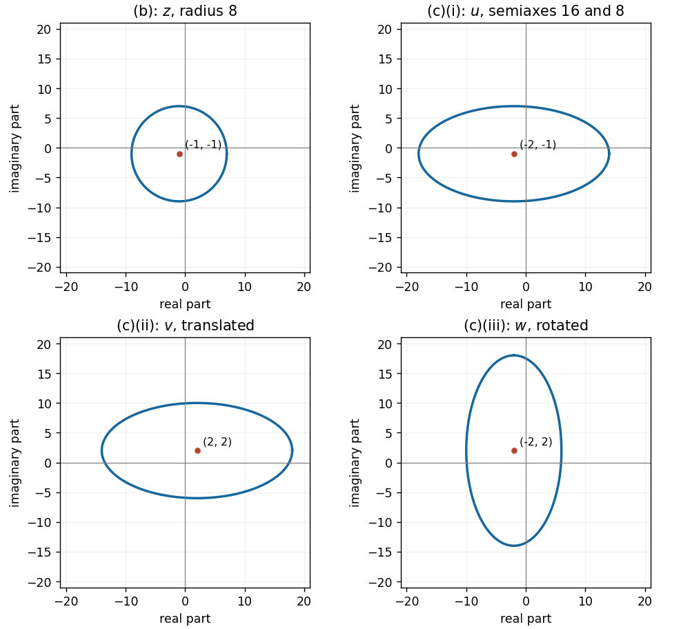
The complex modulus $|z-(-1-i)|$ is the Euclidean distance from $z$ to $-1-i$. Thus the locus isa circle with centre $(-1,-1)$ and radius $8$. Its extreme horizontal coordinates are $-9$ and $7$, and its extreme vertical coordinates are also $-9$ and $7$.

The radial coordinate in the cylindrical coordinate system is the Euclidean distance from the $z$-axis:

The circles have centres $(1,1)$ and $(-1,1)$. Their Euclidean distance is

For the grounded wall, use an image charge $-q$ at $(2b,0)$. Define the Euclidean distances $r=\sqrt{x^2+y^2}$ and $r_{\ast }=\sqrt{(x-2b{)}^2+y^2}$. The method of images givesThe real source has the required Dirac delta function coefficient, and the image is outside the domain. On $x=b$, $r=r_{\ast }$, so $V_D=0$ exactly. This verifies the Dirichlet boundary condition rather than only its derivative.

Choose the polar axis in the source integration along the evaluation vector $r$. The Euclidean distance then satisfies $|r-r^{\prime }{|}^2=r^2+r^{\prime 2}-2r{r}^{\prime }\cos {\theta }^{\prime }$, givingFor the uniform ball, integrate its Newtonian gravitational potential in these spherical coordinates. With $\mu =\cos {\theta }^{\prime }$,For $r,r^{\prime }>0$, the inner integral isobtained from the antiderivative $-\sqrt{r^2+r^{\prime 2}-2r{r}^{\prime }\mu }/(r{r}^{\prime })$. ThereforeFor $0<r<R$, split the radial integral at $r^{\prime }=r$. Its two pieces are ${\int }_0^{r}2r^{\prime 2}d{r}^{\prime }/r=2r^2/3$ and ${\int }_r^{R}2r^{\prime }d{r}^{\prime }=R^2-r^2$. The Newtonian gravitational potential of a uniform solid sphere is consequentlyThe centre value follows by continuity, removing the intermediate $1/r$. For $r>R$, the same integral gives $-GM/r$, so both the potential and first derivative match at the surface. Finally ${\nabla }^2\Phi =4\pi G\rho$ inside, while $-\nabla \Phi =-GM\mathbf{r}/R^3$ is directed inward and vanishes at the centre, checking the sign and normalization.

Let the evaluation point be ${\mathbf{r}}_0=(x,y,z)$, $z>0$, and reflect it to ${\mathbf{r}}_0^{\ast }=(x,y,-z)$. The method of images constructsThe two Euclidean distances coincide on the plane, so $G=0$ there. The negative image source lies outside the domain; inside, only the real source contributes to $-{\nabla }_{\mathbf{r}}^{2}G={\delta }^{(3)}(\mathbf{r}-{\mathbf{r}}_0)$. The difference also decays at infinity.

On the plane write $\mathbf{r}=(\xi ,\eta ,s)$ and set $s=0$. The outward unit normal of the upper half-space is $n=-e_z$. Direct differentiation givesSubstituting into the boundary representation from part (c) yields the Poisson kernel for the upper half-space:Its sign is positive, as expected from the maximum principle for nonnegative boundary data. Its normalization can be checked in polar coordinates:As $z\downarrow 0$ the kernel is an approximate identity, recovering $f$ at its continuity points. Boundary data must have the decay and regularity compatible with the stated condition at infinity.

The domain is the three-dimensional upper half-space. Reflect the source point to ${\mathbf{r}}^{\prime \ast }=(x^{\prime },y^{\prime },-z^{\prime })$. The method of images places an opposite source at this reflected point, giving the Dirichlet image kernel for the three-dimensional modified Helmholtz equationOn $z=0$, the two Euclidean distances are equal, so the terms cancel exactly. The image lies outside the domain, so its contribution satisfies the homogeneous modified Helmholtz equation everywhere inside; only the original source contributes a Dirac delta. Both terms decay at infinity, including for $k=0$, and the homogeneous Dirichlet boundary condition follows.

By translation and rotation invariance, use a radial Green function $G(R)$, where $R=|\mathbf{r}-{\mathbf{r}}^{\prime }|$ is the Euclidean distance. Away from the source, the radial modified Helmholtz equation isWriting $u=RG$ reduces this to $u^{\prime \prime }-{\kappa }^{2}u=0$, where $\kappa =|k|$. For $\kappa >0$, decay eliminates $e^{\kappa R}/R$, leaving $G=A{e}^{-\kappa R}/R$. For $\kappa =0$, the two radial branches are a constant and $1/R$; decay again leaves $A/R$.

To fix the singular normalization, integrate the defining equation over a ball of radius $\epsilon$ about ${\mathbf{r}}^{\prime }$. The divergence theorem givesThe volume term is $O({\epsilon }^2)$, whereasConsequentlySource qualification. The printed $e^{-kR}$ is the decaying branch only when $k\ge 0$, although the source declares $k$ real. For negative $k$ it grows, so it cannot be the requested decaying Green function. The absolute value above covers every real $k$ and reduces to the printed form for nonnegative $k$.

Write $s=|{\mathbf{r}}^{\prime }|$ and ${\mathbf{r}}^{\prime \prime }=a^2{\mathbf{r}}^{\prime }/s^2$. If $|\mathbf{r}|=a$, expansion of squared Euclidean distances givesConsequently $|\mathbf{r}-{\mathbf{r}}^{\prime \prime }|=(a/s)|\mathbf{r}-{\mathbf{r}}^{\prime }|$, and the two terms in $H$ cancel. This method of images gives the Dirichlet Green function inside a sphere:The image point is outside the sphere, so only the physical source contributes a Dirac delta distribution inside. As $s\to 0$, the image position tends to infinity and its coefficient also diverges, but their ratio has the finite limitThusThe apparent singularity of the image construction at a central source is removable; the physical source singularity at $\mathbf{r}=0$ remains.

Let $s=|{\mathbf{r}}^{\prime }|>0$ and $\mathbf{p}={\mathbf{r}}^{\prime }/s^2$. For $|\mathbf{r}|=1$, expanding both squared Euclidean distances givesTaking nonnegative square roots provesThis is the distance identity behind inversion in a circle and the method of images for a circular boundary.

Set $g_j=G_{1/L}(x^j)$, $r_j=\Vert x^j-x^{\ast }{\Vert }^2$ and ${\delta }_j=\varphi (x^j)-\varphi (x^{\ast })$. Here $g_j$ is the proximal gradient mapping, $r_j$ is a squared Euclidean distance, and ${\delta }_j\ge 0$ because $x^{\ast }$ is a global minimizer. The update gives $x^{j+1}=x^j-g_j/L$.

First use the supplied inequality (1) with $z=x^j$:Thus the objective function values, and hence the errors ${\delta }_j$, are nonincreasing. Next use (1) with $z=x^{\ast }$:Expansion of the squared Euclidean norm givesso the last bound is exactly ${\delta }_{j+1}\le L(r_j-r_{j+1})/2$.

The telescoping sum over $j=0,\dots ,k-1$ therefore givesSince each summand is at least ${\delta }_k$, we obtain the proximal gradient objective error boundThe bound holds for the last iterate. The monotonicity of the objective function values is what converts an averaged estimate into this last-iterate estimate.

Let $d=y-x$ and take $0<t\le 1$. Rearrange the defining inequality for a strongly convex function, applied to $x+td$:Because $f$ is differentiable at $x$, its directional derivative in direction $d$ isTaking the limit in the rearranged inequality givesThis is the supporting affine function inequality strengthened by a positive squared Euclidean distance. Differentiability at $x$ alone suffices; no derivative at $y$ is used.

Condition on $X^k=x$, and set $r=x-x^{\ast }$, $g=\nabla f(x)$ and $h=\nabla f_{S_k}(x)$. Since the sampled index is independent of $X^k$ and has the discrete uniform distribution, $h$ is an unbiased stochastic gradient:Write ${\sigma }_k^2=\mathbb{E}[\Vert h-g{\Vert }^2\mid X^k=x]\le M$. Expanding $h=g+(h-g)$ and using the zero conditional mean of $h-g$ proves the stochastic gradient second-moment identityThe stochastic gradient descent update is $X^{k+1}=x-h/L$. Expanding the squared Euclidean distance and using the preceding identities givesThe subgradient inequality for the differentiable convex function $f$ gives $f(x)-f(x^{\ast })\le g^{T}r$. Combining this with (3),Removing the temporary notation for the conditioning point yieldsThe noise contributes twice in this argument: once in the supplied bound (3), and once in converting the expected squared step into the squared gradient. Each contribution is at most $M/(2L)$.

The printed distance needs a square. The native PDF, paper page 3, prints $\Vert x^0-x^{\ast }\Vert$ in the final bound, but the general conclusion from (5) contains $\Vert x^0-x^{\ast }{\Vert }^2$. We first prove the corrected statement and then show that the printed version can fail.

Take the expectation in (5), use the tower property, and sum over $j=0,\dots ,k-1$. The squared Euclidean distances form a telescoping sum:Discard the final nonnegative squared Euclidean distance. The smallest of $k$ numbers is at most their arithmetic mean, soThis is an $O(k^{-1})$ bound above the stochastic gradient noise floor $M/L$ for the best expected objective function value. By Jensen's inequality, it also bounds $\mathbb{E}f({\bar{X}}^k)-f(x^{\ast })$ for the averaged iterate ${\bar{X}}^k=k^{-1}{\sum }_{j=0}^{k-1}{X}^{j+1}$, because $f$ is a convex function.

To test the printed version, take one component function, $f_1(x)=f(x)=x^2/4$, with $L=1$, $x^{\ast }=0$ and $x^0=10$. This convex quadratic function has $\nabla f(x)=x/2$, hence it has a $1$-Lipschitz gradient. The stochastic gradient descent update is deterministic, its conditional variance is zero, and the assumed positive bound $M=1/10$ is valid. At $k=1$, the new iterate is $X^1=5$, soThus the printed inequality is false under its stated assumptions. The squared Euclidean distance in the corrected bound resolves the defect.

An isometry of the Euclidean plane is a map $T:{\mathbb{R}}^2\to {\mathbb{R}}^2$ preserving all Euclidean distances, $\Vert T(x)-T(y)\Vert =\Vert x-y\Vert$. Such a map of the whole plane is automatically bijective, and has the form $T(x)=Rx+b$ with $R$ an orthogonal matrix.

The classification is identity, translations, rotations about a point, reflections in a line, and glide reflections. Here a glide reflection is a reflection followed by a nonzero translation parallel to its mirror. The cases preserving orientation have $\det R=1$ and are translations or rotations; the orientation-reversing cases have $\det R=-1$ and are reflections or glide reflections. The identity is included by allowing a zero translation or rotation angle.

An isometry of the Euclidean plane is a map $T:{\mathbb{R}}^2\to {\mathbb{R}}^2$ preserving all Euclidean distances, $\Vert T(x)-T(y)\Vert =\Vert x-y\Vert$. Such a map of the whole plane is automatically bijective, and has the form $T(x)=Rx+b$ with $R$ an orthogonal matrix.

The classification is identity, translations, rotations about a point, reflections in a line, and glide reflections. Here a glide reflection is a reflection followed by a nonzero translation parallel to its mirror. The cases preserving orientation have $\det R=1$ and are translations or rotations; the orientation-reversing cases have $\det R=-1$ and are reflections or glide reflections. The identity is included by allowing a zero translation or rotation angle.

The age difference is the difference between proper times along two worldlines joining the same departure and reunion events. In the inertial Earth frame a traveler who spends total coordinate time $T$ moving at speed magnitude $v$, with negligible-duration turnaround, accumulates $T\sqrt{1-v^2/c^2}$ while the stay-at-home clock accumulates $T$. These are invariant readings at reunion. Acceleration permits the change of traveling inertial frame, but the result is determined by the whole path, not a universal rule that acceleration itself slows clocks.

Relativity of simultaneity is important when explaining the same result using the traveler's successive inertial coordinates. At the turnaround, the traveler changes which distant Earth event is assigned the same time. The simultaneity slice changes, producing a jump in the coordinate time attributed to Earth in the ideal instantaneous limit. On each long inertial leg the traveler can assign a slow rate to the distant Earth clock without contradicting Earth's larger total elapsed time, because those assignments do not cover the reunion comparison with a single simultaneity convention.

The key distinction is between explaining a coordinate-based apparent symmetry and deriving an invariant result. One can calculate both proper-time integrals in one inertial frame without ever using the traveler's simultaneity jump. Conversely, claiming that each twin must simply see the other younger confuses two reciprocal comparisons between different sets of simultaneous distant events. Radar signals and Doppler shifts provide an operational account with finite signal travel times and the same reunion readings.

Thus relativity of simultaneity resolves a specific misleading inference in the paradox, but is not an extra physical mechanism that changes a clock at a distance. The worldline asymmetry and the invariant proper-time calculation suffice for the prediction; simultaneity explains why reciprocal inertial time-dilation statements cannot be pasted together indiscriminately.^[ref]

The geometrical explanation uses $d{\tau }^2=d{t}^2-d{\mathbf{x}}^2/c^2$ along each timelike path. In flat spacetime an inertial path between fixed timelike endpoints locally maximizes proper time, unlike the familiar shortest-path property of Euclidean distance. This is a physical metric property tested by clocks, not an appeal to a diagram alone. The explanation is satisfactory insofar as it connects that metric, specified worldlines and actual clock behavior; it does not require an absolute flow of time or a special clock-damaging action at the turnaround.

False. Take the metric space $X=\mathbb{R}\times \{0,1\}$ with the Euclidean distance and subspace topology inherited from ${\mathbb{R}}^2$. For every $t\ne 0$, identify $(t,0)$ with $(t,1)$; leave the two points $(0,0)$ and $(0,1)$ in separate equivalence classes. All equivalence classes have one or two points, so all are closed in this metric space.

Let $o_0,o_1$ be the two distinct images of the origins. If $U_0,U_1$ are any open neighbourhoods of $o_0,o_1$ in the quotient space, their preimages contain respectivelyfor some $\epsilon ,\delta >0$. Choose $0<t<\min (\epsilon ,\delta )$. The common image $p(t,0)=p(t,1)$ belongs to both $U_0$ and $U_1$. Therefore the origins have no disjoint open neighbourhoods and the quotient space is not Hausdorff. This is the line with two origins.

The Euclidean distance isThus $d((x,y),(u,v))=\sqrt{(x-u{)}^2+(y-v{)}^2}$. The type synonym expands to pairs of floating-point coordinates.

First include the closing edge exactly once:The recursive version and right fold both sum the Euclidean distances between consecutive vertices, including the last-to-first pair. They take linear time. The empty-list convention gives zero, although an empty list is not a valid polygon.