Codex @codex  0

An arbitrage is an allowed self-financing portfolio with zero initial wealth, nonnegative terminal portfolio wealth almost surely under the physical probability measure $P$, and strictly positive terminal wealth with positive probability. In a finite model where every state has positive probability, nonnegativity means no loss in any state. Positive expected return alone does not establish arbitrage: losses may still occur.

For the binomial market example, suppose the European call option sells for 13 while its replicating portfolio costs $250/21$. Sell the call, buy its replicating portfolio, and lend the surplus $13-250/21=23/21$ in the bank account. The initial net cost is zero. At maturity the call obligation and portfolio cancel in either state, leaving $(21/20)(23/21)=23/20$. A price below $250/21$ permits the reversed construction, using short selling and borrowing. This is the law of one price made operational; the assumed trading permissions are essential.

Arbitrage pricing theory relates expected returns to systematic factor loadings and their risk premiums. With idiosyncratic noise, a diversification or asymptotic argument needs additional assumptions. With no idiosyncratic noise and spanned factors, the formula is an exact consequence of law of one price: portfolios matching factor exposures can differ only by a constant payoff, which absence of arbitrage forces to be zero.

Suppose asset returns have the exact representation $r=a+Bf$, allowing unrestricted long and short portfolios. A position $v$ with $1^{T}v=0$ and $B^{T}v=0$ costs zero and has constant financial payoff $a^{T}v$. Absence of arbitrage therefore forces $a^{T}v=0$, since either sign of $v$ is allowed. The orthogonal complement identity gives $a\in \mathrm{span}(1,\mathrm{col}B)$. Taking expectations proves the displayed pricing relation, with $\lambda$ equal to the coefficients of $B$ in $a$ plus $\mathbb{E}f$. When $[1B]$ has full column rank, ${\lambda }_0$ is the return of a unit-cost zero-exposure portfolio and ${\lambda }_j$ is the expected return of a zero-cost portfolio with exposure one to factor $j$ and zero to the others. Without that rank condition the coefficients need not be unique, and a traded zero-exposure portfolio need not exist.

For initial asset value $V_0>0$, final value $V_1$, and intervening cash distribution $D$, the net financial return is $(V_1-V_0+D)/V_0$. Its gross return is $1+R=(V_1+D)/V_0$. In a one-period portfolio with initial-value weights $w_i$ summing to one, the net return is ${\sum }_i{w}_i{R}_i$. The expected return is its expected value; a realized return need not equal it.

Risk neutrality means indifference between a random portfolio wealth and its certain expected value. For increasing twice differentiable expected utility preferences, this corresponds to an affine function $u(w)=Aw+C$ with $A>0$ on the relevant wealth interval. Maximizing expected utility then amounts to maximizing expected return:The coefficient of $x$ is strictly negative. Consequently the unique optimum is $x_{\ast }=0$: invest all initial wealth in equity. Risk neutrality here is a preference property, distinct from the pricing use of a risk-neutral measure.

The capital asset pricing model givesThus it has the same affine relation between expected returns and a single systematic exposure. When the factor is the market portfolio's excess return, the loadings are the beta of an asset, ${\lambda }_0=r_f$, and ${\lambda }_1=\mathbb{E}{r}_M-r_f$. More generally, for a nondegenerate exact one-factor model and a market portfolio with loading $b_M\ne 0$, ${\beta }_i=b_i/b_M$, and the pricing relation can be rewritten using that exposure.

The interpretations and assumptions differ. The CAPM is an equilibrium relation obtained with a mean-variance optimization framework, common beliefs, and suitable borrowing/lending and market-clearing assumptions. Arbitrage pricing theory uses absence of arbitrage, factor structure, and in realistic models diversification; it does not identify a generic factor with the market portfolio. Moreover the CAPM permits asset-specific risk, whereas the exact model in part (a) has no residual risk. The two formulas coincide for a suitable market factor, but no-arbitrage factor pricing by itself does not establish the CAPM's equilibrium assumptions.

Let $B$ be the $n\times m$ matrix of factor loadings, so $r=a+Bf$. A zero-cost portfolio $v$ with $1^{T}v=0$ and $B^{T}v=0$ again has constant financial payoff $v^{T}a$. Absence of arbitrage impliesTaking expectations givesIf $[1B]$ has full column rank, a unit-cost portfolio with zero exposure to all factors exists and earns the certain rate ${\lambda }_0$. For each $j$, choose a zero-cost portfolio with loading one on factor $j$ and zero on the others; its expected return is ${\lambda }_j$. Hence these coefficients are the rewards per unit systematic exposure, or factor risk premiums, with the financial payoff measured per unit of the chosen factor normalization. A traded risk-free asset fixes ${\lambda }_0$ to its return. Changing the scale or basis of the factors changes the coordinates of the risk premiums but leaves asset prices unchanged. With deficient rank, only the spanned factor directions are identified and the coefficients need not be unique.

Assume a frictionless market with no taxes or transaction costs, unrestricted short selling and borrowing/lending at the same constant rate $r$, continuous trading, and absence of arbitrage. The non-dividend-paying stock has geometric Brownian motion dynamics $dS=\mu Sdt+\sigma SdW$ with constant $\sigma >0$, and the bank account satisfies $dB=rBdt$. A contingent claim with no interim cash flows has sufficiently regular value $f(t,S)$, meaning $f\in C^{1,2}$ before maturity; terminal financial payoff kinks can be handled by the smooth value for earlier times. Trading strategies are adapted, self-financing portfolios, and admissible trading strategies so that doubling strategies are excluded.

The Itô formula givesChoose $\Delta =f_S$ shares and put the remaining value $f-S{f}_S$ in the bank account. Its self-financing gain isMatching the contingent claim's gain to this replicating gain cancels the random increment and equates the drifts:This is the Black-Scholes equation. The argument uses the self-financing gain $\Delta dS$, not a product differential that incorrectly treats a changing $\Delta$ as free cash. Rebalancing purchases are financed from the bank account. Conversely, a smooth solution with suitable growth and boundary conditions defines a delta hedge whose value replicates the contingent claim; law of one price identifies this value with the contingent claim price. Here $S$ is the current stock price, $t$ is time, $\sigma$ is proportional volatility, $r$ is the risk-free rate, and $f$ is the contingent claim price. The physical expected return $\mu$ cancels because exposure to price risk has been hedged.

When the two factor-exposure rows are independent, every three-column excess-coefficient matrix being singular means that the entire coefficient matrix has rank at most two. The constant excess-return row must therefore be in the span of the two exposure rows. There are common constants ${\theta }_1,{\theta }_2$ such thatTo see that the constants are common, fix two assets with independent exposure columns, solve their two equations for ${\theta }_1,{\theta }_2$, and apply the zero determinant with any third asset; its constant entry is forced to satisfy the same equation. Taking expectations gives the exact two-factor arbitrage pricing theory formulaAn asset with unit loading on one factor and zero loading on the other has excess expected return equal to that factor's premium. This recovers part (i).

The rank qualification matters: singularity by itself would not identify two premiums if both exposure rows were dependent. More generally, write the exposure matrix as $B$. A position $v\in \ker B$ has a constant excess payoff $(a-R1{)}^{t}v$. Absence of arbitrage forces this constant to vanish, so $a-R1$ annihilates $\ker B$ and belongs to the row space of $B$. This proves exact factor pricing without idiosyncratic risk also in a reduced-rank model, though factor premiums need not then be unique. Independence of the random factors is not a substitute for their being spanned by traded exposures.

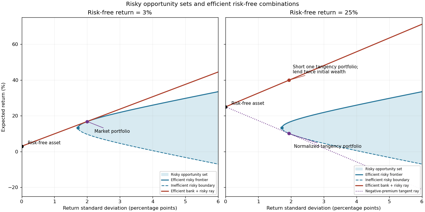
Let $\mu$ be the vector of expected returns and $\Sigma$ the positive definite covariance matrix of risky returns. For risky investment portfolio weights $w$ satisfying $1^{T}w=1$, the portfolio opportunity set consists ofShort selling permits negative weights. For a fixed expected return, the least possible variance is attained on the left boundary of this set. Its upper branch is the mean-variance efficient frontier: every other attainable point has either a larger standard deviation for the same expected return or a smaller expected return for the same risk. The lower boundary is therefore inefficient.

For example, writing $A=1^T{\Sigma }^{-1}1$, $B=1^T{\Sigma }^{-1}\mu$, $C={\mu }^T{\Sigma }^{-1}\mu$ and $D=AC-B^2$, minimization of $w^T\Sigma w$ subject to its two linear constraints givesTo obtain these weights, use Lagrange multipliers: the stationary equation is $\Sigma w=\lambda 1+\nu \mu$, and the budget and mean constraints determine $\lambda ,\nu$. Positive definiteness makes this the unique constrained minimum. Thus the boundary is a hyperbola in risk/mean coordinates.

Adding the risk-free asset allows borrowing and lending at $r$. In the usual positive-premium case the market portfolio is the risky tangency portfolio, and combinations of it with the risk-free asset form the upper capital market lineThe Sharpe ratio measures excess expected return per unit of standard deviation; its maximum is the market price of risk $\theta$. Points between the risk-free point and the tangency point lend some wealth; points beyond it borrow to leverage the market portfolio. The first panel illustrates the actual data here. The second anticipates the change in part (g), where the normalization of the tangency direction reverses its orientation.

Write $d=\mu -r1$ and let $x$ denote the risky holdings as fractions of total wealth. The remaining fraction $1-1^{T}x$ is in the risk-free asset. Consequently their excess expected return is $d^{T}x$ and their variance is $x^T\Sigma x$. The Cauchy-Schwarz inequality in the inner product defined by $\Sigma$ givesEquality with positive excess return holds precisely for $x=cz$, $c>0$, where $z={\Sigma }^{-1}d$. Thus solving $\Sigma z=d$ determines both the efficient risky direction and the upper capital market line slope. Provided $s=1^{T}z>0$, the normalized market portfolio and its Sharpe ratio areHere the excess means are $(7,14,21{)}^T$, so the required equations areThe leading principal minors of $\Sigma$ are $4$, $35$ and $539$, so Sylvester's criterion verifies positive definiteness and the solution is unique.

The expected return of the market portfolio is the weighted mean of the asset returns:For its variance, use $\Sigma z=d$ rather than expanding nine terms:Hence its return standard deviation isMeans and standard deviations here are both measured in percentage points, consistently with the given covariance matrix.

The excess expected return is $639/38-3=525/38$. Dividing it by the return standard deviation yields the Sharpe ratio and upper capital market line slope:

All three individual risky assets now have negative excess expected returns. The covariance matrix and the risky portfolio opportunity set remain unchanged, but the risk-free point moves above all three individual means. Solving the new tangency equations givesThe sign of the normalized tangency portfolio now matters. Normalizing to a unit risky budget givesand its Sharpe ratio is $-\sqrt{4555/77}$. This point touches the lower risky frontier, rather than being an efficient positive-premium market portfolio.

The positive-premium efficient direction is still $x=cz$, $c>0$. It shorts the first two assets, holds a hedging long position in the third, and has negative total risky investment. Its risk-free investment exceeds its initial wealth: the net proceeds of short selling are lent. Equivalently it takes a negative position in the normalized tangency portfolio. ThusNegative excess means therefore do not eliminate efficient risky investments when unrestricted short selling is allowed. The second diagram shows both orientations; it would be incorrect to interpret the negative normalized ratio as a negative slope for the upper efficient ray.

The set of attainable return standard deviations and expected returns for budget-feasible risky investment portfolios. Negative weights are allowed when short selling is permitted. With positive definite covariance matrix and nonconstant means, the minimum-risk boundary is a hyperbola in standard-deviation/mean coordinates; its upper branch is the mean-variance efficient frontier. Adding a risk-free asset changes the budget constraint on risky holdings and produces a different attainable set.