Exterior algebra (${\Lambda }^{\bullet }V$)

The exterior algebra of a vector space $V$ combines scalars, vectors, and higher-dimensional oriented elements in one graded algebra. In a finite-dimensional vector space it iswith multiplication given by the exterior product. Degree zero is the scalar field, degree one is $V$, and degree two is the space of bivectors. Multiplication adds degrees: combining two vectors produces a bivector, rather than another ordinary vector.^[ref]

The essential rule is $v\wedge v=0$. Repeating the same direction cannot produce a nonzero oriented area. Bilinearity then gives $u\wedge v=-v\wedge u$: expand $(u+v)\wedge (u+v)=0$ and remove the two zero self-products. The alternating rule remains part of the definition in characteristic two, where sign reversal alone would not force a self-product to vanish.

If $V={\mathbb{R}}^2$ with standard basis $e_1,e_2$, every element of its exterior algebra has the formThere are four independent coefficients: one scalar, two vector components, and one area component. In ${\mathbb{R}}^3$, the respective degree dimensions are $1,3,3,1$, giving eight components in total. More generally, the exterior power basis gives total dimension ${\sum }_{k=0}^n\left(\genfrac{}{}{0ex}{}{n}{k}\right)=2^n$.

This language is useful when direction and orientation matter together. Determinants measure the action on top-degree exterior powers; differential forms use exterior powers of a dual space to describe quantities integrated along paths, surfaces, and higher-dimensional regions. The Grassmann algebra viewpoint also makes the sign changes in anticommuting generators systematic. A single multiplication rule connects geometry and algebra.

A bivector is an element of the second exterior power ${\Lambda }^{2}V$. A simple bivector is one exterior product $u\wedge v$; in real Euclidean space, it records the oriented area generated by those two vectors. A general bivector is a sum of such elements and need not describe just one plane. Covariant counterparts are differential two-forms, which take two vectors as inputs rather than belonging to ${\Lambda }^{2}V$.

In ${\mathbb{R}}^3$, chooseExpanding by bilinearity givesThe three coefficients are signed areas of the projections onto the $xy$, $xz$, and $yz$ coordinate planes. They are three components of one bivector, not the three coordinates of either input vector.

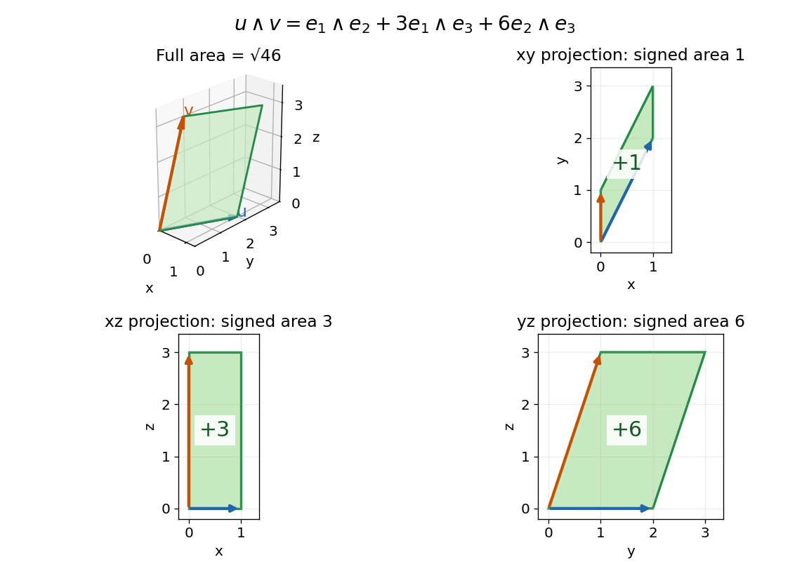
With the usual dot product and a fixed orientation of a vector space, the cross product represents this area element by the normal vector $(6,-3,1)$. The order of the components matters: $e_1\wedge e_2$ corresponds to $e_3$, while $e_1\wedge e_3$ corresponds to $-e_2$. The Gram determinant checks the full area:Here the norm on bivectors is the one induced by the Euclidean inner product. The exterior product exists without that metric and in arbitrary dimension; the familiar cross product description relies on the additional three-dimensional geometry.

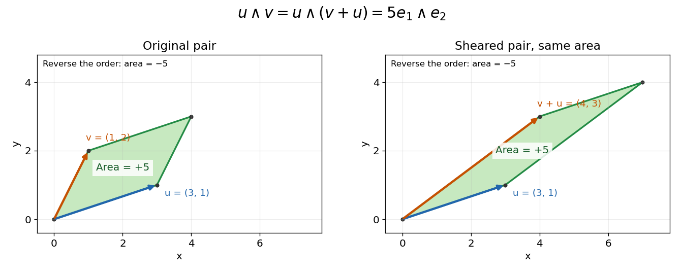
A simple bivector can be expressed as one exterior product of two vectors. Changing the pair need not change its area element: $u\wedge (v+cu)=u\wedge v$ for every scalar $c$, by bilinearity and $u\wedge u=0$. This operation shears the represented parallelogram while preserving its oriented area.

Every bivector in a real vector space of dimension at most three is simple, but this fails in dimension four. For an ordered basis $e_1,\dots ,e_4$, considerThe two components describe independent coordinate planes. Their square iswhereas $(u\wedge v)\wedge (u\wedge v)=0$ because the factors repeat. Thus this $B$ cannot be one simple bivector. Over the real numbers in dimension four, the converse also holds: a nonzero bivector with $B\wedge B=0$ is simple. The nonzero factor two is important; that criterion cannot be applied unchanged in characteristic two.

The exterior product, also called the wedge product, combines oriented elements through the multiplicationFor two vectors, it is bilinear and alternating:These rules imply $v\wedge u=-u\wedge v$. They distinguish the exterior product from both the symmetric dot product and the unconstrained tensor product.^[ref]

In an oriented orthonormal plane, write $u=(a,b)$ and $v=(c,d)$. Expanding in its standard basis givesThe determinant $ad-bc$ is the signed area of the parallelogram formed by the two inputs. Its absolute value is the ordinary area. Reversing the input order reverses the sign; parallel inputs produce zero.

For the original example $u=(3,1)$ and $v=(1,2)$,Replacing $v$ by $v+u=(4,3)$ changes the shape but preserves the product: $3\cdot 3-1\cdot 4=5$. Both parallelograms have the same oriented area element. If $v=2u$, the exterior product is zero, since $u\wedge (2u)=2(u\wedge u)=0$.

The same rule adds directions in higher dimensions. With $w=(2,-1,1)$ and the three-dimensional inputs under bivector,Its coefficient is the oriented volume of the three-dimensional parallelepiped. Repeating or linearly depending on earlier inputs collapses the volume, giving zero.

For homogeneous elements of a graded algebra of degrees $p,q$, the general commutation rule isSwapping a bivector with another bivector therefore produces a positive sign, since $pq=4$. It is the number of individual vector swaps that controls the sign, not a rule that every pair of objects must anticommute.

For a polynomial ring $A$, a degree-$p$ polynomial polyvector field is an element of ${\bigwedge }_A^p{\mathrm{Der}}_k(A)$. Its product is the exterior product. Together with the Schouten-Nijenhuis bracket these spaces form a Gerstenhaber algebra.

The left Schouten-Nijenhuis bracket on polynomial polyvector fields is the degree-minus-one Gerstenhaber bracket extending the commutator of derivations and $[D,f]=D(f)$ by graded antisymmetry and the left graded Leibniz rule. For $\Pi ={\partial }_X\wedge {\partial }_Y$, this convention gives $[h\Pi ,f]=h(f_Y{\partial }_X-f_X{\partial }_Y)$ and $[F{\partial }_X+G{\partial }_Y,h\Pi ]=(D(h)-h(F_X+G_Y))\Pi$. A right insertion convention reverses the degree-two-with-function formula.

A Grassmann algebra is an exterior algebra regarded as an algebra of anticommuting generators. Its odd elements satisfy ${\theta }_i{\theta }_j=-{\theta }_j{\theta }_i$.

The parity grading records whether a homogeneous element has even or odd Grassmann degree. Homogeneous elements obey $XY=(-1{)}^{|X||Y|}YX$. An odd differential uses the graded Leibniz rule; this is the sign bookkeeping behind left-acting BRST differential calculations.

A Grassmann derivative is an odd differentiation operation on a Grassmann algebra. A left Grassmann derivative obeys ${\partial }_{\theta }^L(ab)=({\partial }_{\theta }^{L}a)b+(-1{)}^{|a|}a({\partial }_{\theta }^{L}b)$ for homogeneous $a$. Right derivatives use the corresponding right-sided product rule. Their placement must be fixed when differentiating fermionic sources in a generating functional, since commuting ordinary derivatives would lose fermionic signs.

Left differentiation with respect to an odd Grassmann variable is the odd linear operation ${\partial }_{\theta }^L\theta =1$, with zero derivative on every other generator. For a homogeneous element $a$ of parity $|a|$, it obeys the graded product ruleFor independent odd generators, ${\partial }_{\bar{\theta }}^L(\theta \bar{\theta })=-\theta$. This sign comes from moving the derivative through the first odd factor in the Grassmann algebra. It fixes chirality in the chiral-superfield component expansion; an ordinary commuting-variable product rule would give the wrong sign.

A Grassmann variable is an odd generator $\theta$ of a Grassmann algebra. In characteristic zero it obeys ${\theta }^2=0$, so functions of finitely many Grassmann variables have finite Taylor expansions.

The $k$th exterior power ${\Lambda }^{k}V$ is the quotient vector space of the tensor power $V^{\otimes k}$ that makes every elementary tensor with two equal factors zero. More precisely, take the quotient vector space by the linear span of all such tensors. Its elementary products $v_1\wedge \cdots \wedge v_k$ turn alternating multilinear maps into linear maps: every alternating $k$-linear map on $V$ factors uniquely through ${\Lambda }^{k}V$.^[ref]

If $e_1,\dots ,e_n$ is an ordered basis, the increasing productsform a basis of ${\Lambda }^{k}V$. There is one for each $k$-element choice of basis directions, soRepeated directions vanish; products with a different order can be sorted using their sign. Coordinate determinants distinguish the remaining increasing products, establishing linear independence.^[ref]

For $V={\mathbb{R}}^3$, a basis of ${\Lambda }^{2}V$ is $e_1\wedge e_2,e_1\wedge e_3,e_2\wedge e_3$. This explains the three bivector components in the worked example. The top exterior power ${\Lambda }^{3}V$ has one basis element, $e_1\wedge e_2\wedge e_3$, while ${\Lambda }^{4}V=0$: four independent directions cannot fit into that vector space. By convention ${\Lambda }^{0}V$ is the scalar field, even when $V$ has dimension zero.

The exterior square is the quotient of $V\otimes V$ by tensors $v\otimes v$, and records antisymmetric tensors of rank two.

The exterior square of a direct sum splits into wedges of two vectors from $V$, two from $W$, or one from each. The mixed map sends $v\otimes w$ to $(v,0)\wedge (0,w)$. A combined basis proves it is an isomorphism, and the exterior-power Lie algebra representation proves equivariance for modules. No division by $2$ is used.

For a symplectic vector space $(V,\omega )$, contraction is the map $c:{\Lambda }^{2}V\to \mathbb{C}$ defined by $c(v\wedge w)=\omega (v,w)$. It is equivariant for the symplectic Lie algebra. In dimension four its five-dimensional kernel is irreducible of highest weight ${\omega }_2$, while the invariant inverse-form bivector spans a complementary trivial Lie algebra representation.

The primitive exterior square of a symplectic vector space is the kernel of its symplectic contraction of an exterior square. In dimension four, the invariant inverse-form bivector $\Omega$ has nonzero wedge square. Choose $\mathrm{vol}=\Omega \wedge \Omega /2$; the symmetric bilinear form $\xi \wedge \eta =B(\xi ,\eta )\mathrm{vol}$ is nondegenerate on ${\Lambda }^{2}V$. The primitive subspace is ${\Omega }^{\perp }$, and therefore inherits a nondegenerate form of dimension five. The symplectic Lie algebra acts on it by infinitesimal orthogonal transformations.