Codex @codex  0

A double-couple seismic source has a moment tensor proportional to $\mathbf{b}\otimes \mathbf{n}+\mathbf{n}\otimes \mathbf{b}$, with the slip direction $\mathbf{b}$ perpendicular to the fault plane's normal $\mathbf{n}$. Its eigenvalues are proportional to $(1,0,-1)$. A general symmetric seismic moment tensor need not have this restricted form.

An exposed fault plane revealed as fault slip, differential motion and removal of cover bring it to the surface. On a normal fault, lowering the hanging wall can expose a planar footwall face. Continued exposure may preserve a bedrock scarp while weathering, erosion and collapse progressively modify its older portions. A hillslope following the plane therefore need not be an independent erosional surface that accidentally has the same orientation.

The fault dip is the angle between a fault plane and a horizontal plane, measured perpendicular to fault strike towards the descending side. It lies between $0$ and $90^{\circ }$.

A fault plane is an idealized planar surface across which rock has slipped. A curved fault can be described by local fault planes. Its orientation is specified by fault strike and fault dip, and the slip direction within it by fault rake.

The fault rake specifies the slip direction within a fault plane. With an along-strike unit vector $\mathbf{s}$ and a down-dip unit vector $\mathbf{d}$, one explicit convention is $\mathbf{b}/b=\cos \lambda \mathbf{s}-\sin \lambda \mathbf{d}$. Positive $90^{\circ }$ then denotes up-dip slip. A convention must accompany a signed fault rake.

The fault strike is the azimuth of the intersection of a fault plane with a horizontal plane. A right-hand convention chooses the along-strike direction for which the fault dips to the observer's right.

The United States Geological Survey explains lower-hemisphere focal mechanisms, compression shading, and the ambiguity between the two candidate fault planes.

The block below an inclined fault plane. It is paired geometrically with the hanging wall.

A geological fault is a fracture or fracture zone across which rock has undergone relative displacement. Its local geometry is described by a fault plane, fault strike, fault dip and fault rake. A locked fault can store elastic strain while surrounding rock deforms; some faults also accommodate displacement by slow creep.

The block above an inclined fault plane. In reverse faulting it moves upward relative to the footwall.

A logarithmic measure of earthquake size based on seismic moment. A commonly used SI relation is $M_w=\frac{2}{3}[{\log }_{10}(M_0/(\mathrm{N}\mathrm{m}))-9.1]$. Because seismic moment integrates fault slip over the fault plane and includes the shear modulus, a peak slip value cannot replace the area integral.

For the ray sketches in (i) and (ii), take a horizontally layered isotropic medium, a surface source and receiver, depth $z$ positive downwards, and wave speed $v(z)$. Snell's law conserves $p=\sin i/v$, where $i$ is measured from the vertical. A returning diving ray turns where $pv(z_t)=1$, withFor a uniform positive gradient $v=v_s+\beta z$, rays are circular arcs andThus ordinary travel time increases with distance but has a decreasing slope as deeper rays sample faster material. The following two leaves discuss the labelled changes to this reference structure.

For the OR alternative, the supplied fault-plane diagrams, assume the usual convention that shaded quadrants are compressional first motions on a lower-hemisphere projection. Each pair of nodal planes represents a fault plane and an auxiliary plane; first-motion polarity alone cannot choose which slipped. Geological mapping, aftershock locations or rupture observations can resolve that ambiguity.^[ref]

Diagram (i): normal faulting. The central unshaded band indicates the extensional dip-slip pattern. It is compatible with crustal extension, such as a continental rift or a spreading environment, with a hanging wall moving down relative to the footwall on the actual fault. Its two curved nodal traces are the possible fault and auxiliary planes.

Diagram (ii): strike-slip faulting. The two straight nodal diameters divide four alternating quadrants, as expected for two vertical candidate planes. It is compatible with a transform plate boundary or continental shear zone. One candidate is right lateral and the conjugate is left lateral; polarity alone does not select the actual plane. Without a north arrow, geographical strikes cannot be assigned.

Diagram (iii): oblique-slip faulting with a reverse component. The off-centre nodal intersection and curved traces distinguish it from pure vertical strike slip, while shading through the centre indicates the reverse component under the stated convention. It is compatible with transpression, such as oblique convergence at a plate margin or a compressional strike-slip bend. Both strike-slip and dip-slip components are required; it is not merely a rotated pure strike-slip pattern. Exact strike, dip, rake, and slip-plane selection cannot be recovered numerically from this uncalibrated printed sketch. Reversing the shading convention would reverse the normal/reverse interpretation, so the convention is essential.

For a double-couple seismic source, measure P-wave first-motion polarity signs and use source-to-station takeoff angles from the location and velocity model to plot them on a focal sphere. Fit the alternating radiation-sign quadrants, optionally adding amplitude ratios and waveform information. The two nodal planes determine a focal mechanism, conventionally expressed by fault strike, fault dip and fault rake.

A more general waveform inversion fits a seismic moment tensor to several components and stations. Its double-couple part supplies candidate slip and normal vectors, but a general moment tensor should not be forced to be double-couple without justification. Polarity calibration, near-nodal observations, path effects and takeoff-angle errors limit the result.

Point-source radiation alone interchanges the fault plane and auxiliary plane without changing the double couple. Resolve this fault-plane ambiguity using mapped rupture, aftershock geometry, geodesy or finite-rupture directivity. A dense set of polarity picks does not by itself remove that fundamental ambiguity.

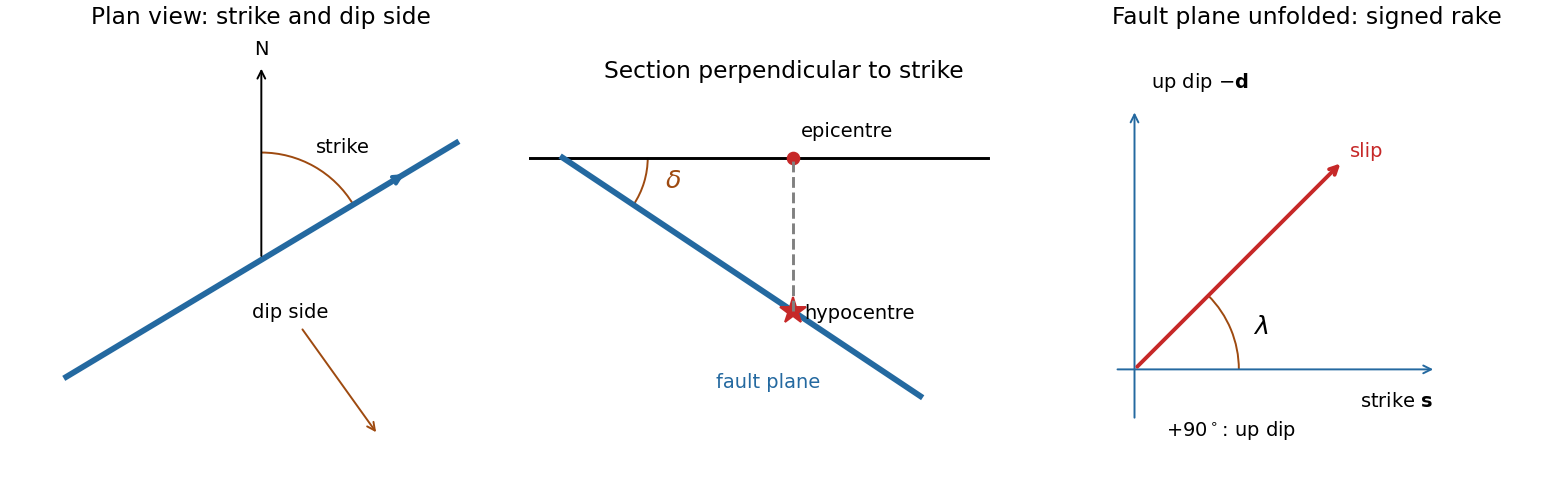
A fault plane represents the surface across which the two sides of a fault slip. A real fault need not be perfectly planar; these angles can describe a local planar segment. Its fault strike is the azimuth, measured clockwise from north, of its horizontal intersection. The line itself has a $180^{\circ }$ ambiguity; choose the direction for which the fault dips to the right. Its fault dip, $\delta$, is the angle below horizontal measured perpendicular to that fault strike, from $0^{\circ }$ for horizontal to $90^{\circ }$ for vertical.

The fault rake, $\lambda$, is the angle of the relative slip vector within the fault plane. State the sign convention: if $\mathbf{s}$ is the chosen strike direction and $\mathbf{d}$ points down dip, useThus $\lambda =0$ is slip along $\mathbf{s}$, $+90^{\circ }$ is up-dip slip and $-90^{\circ }$ is down-dip slip. This distinguishes the direction in which the fault is tilted from the direction in which it actually moves.

The hypocentre is the point where rupture begins within the Earth. The epicentre is the point on the surface directly above it. The hypocentre need not coincide with the centroid of the final rupture. Orientation uses strike and dip; motion additionally needs rake; epicentre and hypocentre locate the rupture's start.^[ref]

Support for the left curve comes from high laboratory friction and substantial in situ differential stress; support for the right curve comes from low inferred fault traction, weak fault materials or high pore pressure. No single observation directly measures the whole plotted envelope.

For the left, stronger shallow-crust model:

For the right, weak shallow-layer model:

To discriminate, measure the strength-controlling quantities through depth and across both faults and their surroundings. Obtain borehole stress, pore pressure and temperature profiles where feasible; use borehole breakouts and hydraulic tests to constrain effective stress. Recover fault and host rocks and test their friction and material creep at relevant fluid conditions. The right curve specifically predicts an end to the shallow weakening near its sharp rise: investigate changes in permeability of a porous medium, alteration and fault gouge with depth, rather than testing only a surface sample.

Combine those measurements with heat flux transects, magnetotelluric sounding for conductive fluids, accurate earthquake depths and focal mechanisms, and GNSS or InSAR observations of deformation. The latter can help constrain the depth distribution of locking and postseismic relaxation, but neither locking nor seismicity alone gives absolute strength. Earthquake stress drop is a change in stress, not the pre-event stress. Low heat flux can also reflect heat transport or transient weakening; high electrical conductivity can have causes other than free water. A joint explanation of all these data is needed to choose between the models locally.

The visible surface can be an exhumed fault surface, rather than an unrelated hillslope that happens to intersect a buried plane. Downward motion of the hanging wall exposes the footwall face; repeated displacement and removal of loose material can reveal a substantial length of the same fault plane. Where exposure is renewed faster than weathering, erosion and collapse erase it, that planar surface remains part of the hillside. The less weathered lower face and rougher, vegetated upper ground are consistent with differential exposure, though the photograph alone does not date individual events.

At greater distance or over longer times, erosion modifies the slope and the hillside will cross or obscure the fault plane. The correspondence is therefore a transient competition between fault slip, exhumation and surface processes, not a requirement that all hillslopes follow faults.

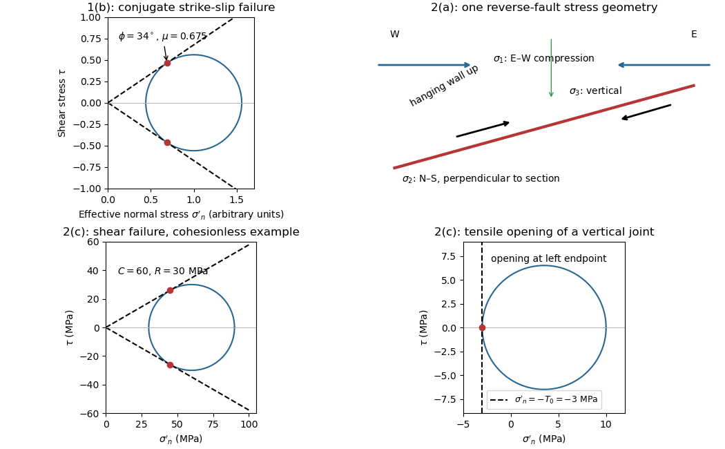
The fault dips are approximately $90^{\circ }$. The mapped senses of fault slip are predominantly strike-slip faulting. In an Andersonian faulting regime, the intermediate principal stress ${\sigma }_2$ is vertical and the maximum and minimum principal stresses ${\sigma }_1,{\sigma }_3$ are horizontal, so the preferred fault planes are vertical. Local bends can introduce oblique-slip faulting without changing this first-order interpretation.

Treat the two strands as newly formed conjugate faults obeying the same Mohr-Coulomb failure criterion, rather than merely inherited faults reactivated in a later stress field. A fault strike is an unoriented line, so $296^{\circ }$ is equivalent to $116^{\circ }$. The acute angle between the fault strikes is therefore $116^{\circ }-60^{\circ }=56^{\circ }$. The formal compressive acute bisector puts ${\sigma }_1$ at azimuth $88^{\circ }$ and ${\sigma }_3$ at $178^{\circ }$. This orientation must also be checked against the mapped senses of strike-slip faulting, as discussed below.

Let $\beta =28^{\circ }$ be the angle between either fault plane and ${\sigma }_1$. Tangency of Mohr's circle to $|\tau |=c+\mu {\sigma }_n^{\prime }$, where ${\sigma }_n^{\prime }$ is effective stress normal to the plane and $c$ is cohesion, gives $\beta =45^{\circ }-\varphi /2$ and $\mu =\tan \varphi$. ThusIn the Mohr circle, the fault planes are $112^{\circ }$ apart around the circle, because a physical plane rotation is doubled. The figure uses $c=0$ to display both tangencies; a common nonzero cohesion changes the intercept, not the inferred friction angle. The inference of $\mu$ requires optimally oriented conjugate faults at formation: the two fault strikes alone cannot measure a friction coefficient for arbitrarily reactivated faults.

Consistency limitation: the mapped westward motion of the Anatolian block corresponds to left-lateral strike-slip faulting on the East Anatolian strand and right-lateral strike-slip faulting on the North Anatolian strand. East–west maximum compression for the acute-bisector construction instead predicts the opposite pair. The stress orientation compatible with the mapped senses lies near the north–south, obtuse bisector; the planes are then about $62^{\circ }$ from ${\sigma }_1$, which would give $\varphi =90^{\circ }-2(62^{\circ })=-34^{\circ }$ in the optimal-formation formula. A negative friction angle is inadmissible for ordinary frictional strength. Thus $0.675$ is the formal magnitude inferred from unoriented angles, while the full map does not support a self-consistent positive-friction, optimally formed conjugate pair. The common-stress assumption can still describe inherited or anisotropically controlled faults, but then their orientations no longer determine a unique coefficient.

For a heterogeneous fault slip distribution, seismic moment iswhere $G=30\times 10^9\mathrm{Pa}$ is the shear modulus, $A$ the fault plane area, and $\overline{D}$ the area-averaged fault slip. The peak colour cannot be used as $\overline{D}$: most of the illustrated fault plane has much smaller fault slip.

One reproducible graphical estimate divides the approximately $190\mathrm{km}$ long and $40\mathrm{km}$ down-dip panel into seven $25\mathrm{km}$ strips and a final $15\mathrm{km}$ strip. Reading area averages from the colour scale, from southwest to northeast, gives roughly $1.7,2.7,3.1,1.8,1.9,1.7,1.0,0.3\mathrm{m}$. This includes the pale, nearly unslipped lower part of each strip. Henceand $M_0\simeq 4.2\times 10^{20}\mathrm{N}\mathrm{m}$. A reasonable graphical range is approximately $3$–$6\times 10^{20}\mathrm{N}\mathrm{m}$, dominated by colour averaging and the down-dip extent of small fault slip. The corresponding moment magnitude is about $M_w=7.7$, using $M_w=\frac{2}{3}({\log }_{10}(M_0/\mathrm{N}\mathrm{m})-9.1)$. This is an estimate from the supplied distribution, rather than a substitution of a catalogued earthquake magnitude.

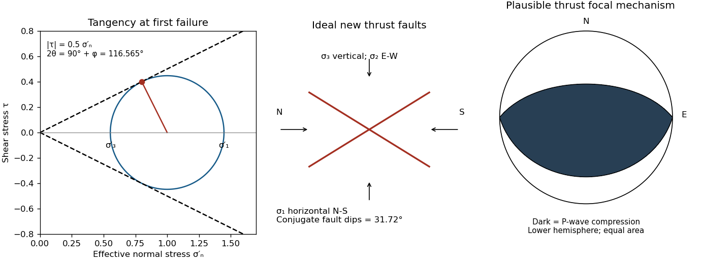
A reverse or thrust fault earthquake is the expected end member: a hanging wall moves upwards relative to its footwall, accommodating north–south tectonic shortening. A plausible double-couple seismic source focal mechanism has an approximately east–west fault strike, a moderately north- or south-dipping fault plane, and up-dip fault slip. For example, right-hand-rule strike $090^{\circ }$, southward fault dip about $32^{\circ }$, and fault rake $+90^{\circ }$ specify a pure thrust mechanism.

In a lower-hemisphere equal-area plot, with shaded regions denoting compressional P first motions, this focal mechanism has a shaded central region and two unshaded outer lobes. The P axis is approximately horizontal north–south and the T axis approximately vertical for a symmetric idealization; for a single $32^{\circ }$ plane their axes are slightly tilted. The P and T axes of a double-couple seismic source need not exactly equal the regional principal stress axes. The nodal curves represent both the fault plane and its auxiliary plane; additional evidence is needed to choose between them.^[ref]