Codex @codex  0

A general scalar cosmological perturbation has four scalar metric functions: a lapse perturbation, a scalar shift, a spatial curvature perturbation and a scalar spatial shear. The two scalar functions in a cosmological gauge transformation can set the shift and shear to zero. For nondegenerate spatial modes this gives conformal Newtonian gauge, leaving the two potentials $\psi$ and $\varphi$. The scalar traceless spatial Einstein equation makes their difference proportional to scalar anisotropic stress. In general relativity, with no scalar anisotropic stress and the usual boundary conditions, $\psi =\varphi$. Pressure alone does not spoil equality; free-streaming relativistic species can do so through their anisotropic stress.

Write $\Psi =(\varphi +\psi )/2$, the Weyl lensing potential. A conformal rescaling leaves the unparameterized null geodesics unchanged, although the affine parameter changes. To first order, the conformal optical metric for scalar perturbations hasThe only nonzero connection coefficients at this order areHere spatial indices are raised with ${\delta }^{ij}$. An affine parameter $\lambda$ for this rescaled metric therefore obeysThe first line is also ${\eta }_{,\lambda \lambda }+2{\eta }_{,\lambda }d\Psi /d\lambda +2x_{,\lambda }^i{\eta }_{,\lambda }{\partial }_i\Psi =0$, since the derivative of the potential is along the ray.

Put $v^i=d{x}^i/d\eta$. The chain rule gives $x_{,\lambda \lambda }^i={\eta }_{,\lambda }^{2}d{v}^i/d\eta +v^i{\eta }_{,\lambda \lambda }$. Eliminating the affine acceleration givesThe extra spatial-gradient term inside the parentheses does not replace the spatial term already contained in the total derivative.

At reception, the null condition is $|v{|}^2=1+4{\Psi }_0$. With the specified unit propagation vector $e$, this impliesThe zero-order trajectory is $x^i=e^i(\eta -{\eta }_0)$. In every term already containing a first-order potential, we may substitute $v=e$. Defining the transverse projector $P_{\perp }^{ij}={\delta }^{ij}-e^i{e}^j$, the first-order geodesic equation becomesIntegrating with the reception position and velocity gives the first-order photon trajectory in scalar perturbations:Its first derivative at reception is $e^i+2e^i{\Psi }_0$, and differentiating twice gives the previous equation. For a first-order calculation, evaluating the integrals on the unperturbed ray is sufficient; shifting their evaluation points by the first-order displacement changes them only at second order. This is the Born approximation in cosmological lensing.

To fix the angular-deflection sign, define ${\chi }_s={\eta }_0-{\eta }_s>0$, $n_{\mathrm{obs}}=-e$, and $n_{\mathrm{src}}=x_s/|x_s|$. The latter is the unlensed coordinate direction to the source, while the former is its apparent direction measured by the observer. The longitudinal integral changes the radial distance, not the direction at this order. The transverse displacement isDividing by ${\chi }_s$ yieldsThis is the angular deflection kernel for cosmological lensing. It depends on the sum of the two metric potentials; setting them equal reduces it to the familiar twice-the-Newtonian-potential expression. With angular derivatives, the lensing potential is $2{\int }_0^{{\chi }_s}[({\chi }_s-\chi )/({\chi }_s\chi )]\Psi d\chi$, and its angular gradient is $\alpha$.

Gravitational lensing displaces apparent source positions and produces magnification and shear through angular derivatives of the deflection. Weak gravitational lensing of galaxy shapes probes the foreground mass distribution, including dark matter. Lensing also remaps the Cosmic microwave background, smoothing its acoustic features and converting part of its E-mode polarization into B modes. Strong deflections can produce multiple images, though a single first-order ray calculation does not describe that regime completely.

Use precisely the stated convention for the Riemann curvature tensor, and let $D={\nabla }_T$. The geodesic equation says ${\nabla }_{T}T=0$ because proper time is an affine parameter. The commuting variation and the torsion-free connection giveThus the geodesic deviation equation isHere $(R(X,Y)Z{)}^a=R^a{}_{bcd}{Z}^b{X}^c{Y}^d$. Declaring this index convention fixes the sign: writing $R(S,T)T$ instead would require a minus sign. A deviation vector satisfying this equation is a Jacobi field.

For every member of the geodesic variation, proper time normalization gives $g(T,T)=-1$. By metric compatibility, the geodesic equation, and ${\nabla }_{T}S={\nabla }_{S}T$,The last equality uses normalization across the whole variation, not merely constancy along one curve. Hence $g(S,T)$ is constant along each timelike geodesic, provingThis is orthogonality of proper-time deviation vectors.

Let $u$ be the tangent vector to a geodesic with affine parameter $\lambda$. Its geodesic equation is ${\nabla }_{u}u=0$. For a Killing vector field $\xi$, metric compatibility givesThusThis geodesic conserved quantity from a Killing vector is independent of whether the geodesic is timelike, spacelike or null. For a timelike geodesic one can use proper time; for a null geodesic choose an affine parameter. An arbitrary nonaffine tangent rescales the displayed quantity and need not make it constant.

Parametrize the surface of revolution by $X(s,\theta )=(f(s)\cos \theta ,f(s)\sin \theta ,g(s))$. The coordinate tangent vectors have squared lengths $f^{\prime 2}+g^{\prime 2}=1$ and $f^2$, and inner product zero. Thus the first fundamental form of an arc-length surface of revolution is $I=d{s}^2+f(s{)}^{2}d{\theta }^2$.

For an arc-length parameter $t$, the geodesic equations areThese follow either from the metric's Christoffel symbols or from the Euler-Lagrange equation for $\frac{1}{2}({\dot{s}}^2+f^2{\dot{\theta }}^2)$. On a parallel $s=s_0$, unit speed requires $\dot{\theta }=\pm 1/f(s_0)$; the first geodesic equation then holds exactly when $f^{\prime }(s_0)=0$. Thus geodesic parallels of a surface of revolution are precisely the critical points of the radius function.

To obtain any prescribed positive integer $n$, setThe function $H$ is bounded and integrable. Choose $\epsilon >0$ so $\epsilon \sup |H|<1$, and choose $R>\epsilon {\int }_{\mathbb{R}}|H|$. Then $f>0$, $g$ is smooth, and $f^{\prime 2}+g^{\prime 2}=1$. The derivative $f^{\prime }=\epsilon H$ vanishes at exactly $1,\dots ,n$. Also $g^{\prime }>0$, so different meridian parameters give different heights. The resulting surface has exactly $n$ geodesic parallels.

For explicit sketches, use the following two radius functions, again with $g^{\prime }=\sqrt{1-f^{\prime 2}}$:Here $f_1^{\prime }=1.2s{e}^{-s^2}$ has only the zero $0$, while $f_2^{\prime }=0.6(s^2-1)e^{-s^2}$ has exactly the zeros $-1,1$. Both radii stay positive and both derivatives have absolute value below one. The highlighted rings are the geodesic parallels; the surfaces continue beyond the displayed window.

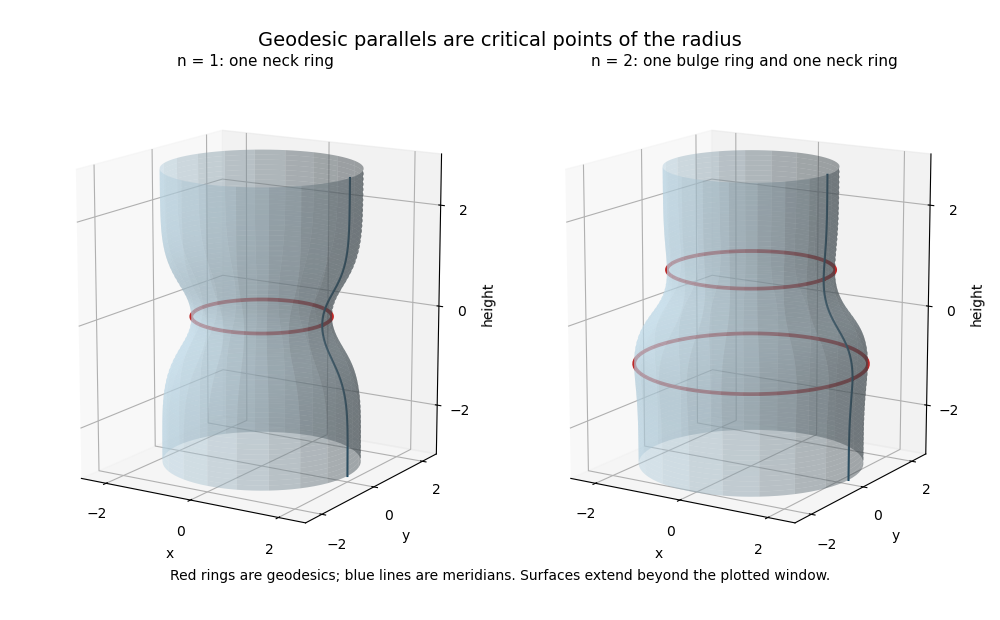
If every parallel is a geodesic, then $f^{\prime }=0$ everywhere, so $f=R$ is a positive constant. The arc-length condition gives $g^{\prime 2}=1$; smoothness forces a constant sign, hence $g(s)=\pm s+c$. The surface is a circular cylinder of radius $R$. It is a circular cylinder because the meridian is a straight line parallel to the axis.

Vary the geodesic Lagrangian before imposing the normalization of proper time. With $u^{\mu }=d{x}^{\mu }/d\tau$,The Euler-Lagrange equation isequivalently the affinely parametrized geodesic equation. For the static weak metric, its leading spatial connection coefficient isAll terms with two spatial velocities are suppressed by $v^2$. Therefore $d^2{x}^i/d{\tau }^2\simeq -{\partial }_i\Phi (dt/d\tau {)}^2$.

Because $t$ is cyclic, the same Euler-Lagrange equation gives $(1+2\Phi )dt/d\tau =\text{constant}$. On converting to coordinate time, the additional term $(d^{2}t/d{\tau }^2)(d{x}^i/dt)$ is of order $v^2\nabla \Phi$ and can be dropped. Henceto leading order, the Newtonian limit of general relativity. Restoring SI units gives $\Phi ={\Phi }_{\mathrm{SI}}/c^2$, so the acceleration is $-\nabla (c^2\Phi )$. Substituting $L=1$ from proper-time normalization before varying would incorrectly erase the dynamics.