Codex @codex  0

A Fourier partial sum retains the modes whose integer frequency multipliers satisfy $|k|\le n$ in a complex Fourier series:For a real function of period $2\pi$, this is equivalently $a_0/2+{\sum }_{k=1}^n[a_k\cos (kx)+b_k\sin (kx)]$. It is a trigonometric polynomial, even when the original function is discontinuous. For a square wave, retaining $M$ nonzero odd sine modes gives $S_{2M-1}f$; all even-frequency coefficients are zero. The Gibbs phenomenon illustrates why more retained modes need not reduce the maximum error.

A Fourier series describes a periodic function through sines and cosines whose frequencies are integer multiples of one base frequency. These Fourier harmonics give a useful alternative to describing the value at every input: each Fourier coefficient measures how much of one oscillating pattern is present. For a real, integrable function of period $2\pi$, the real form isThe cosine formula includes $n=0$; the sine formula uses $n\ge 1$. Thus $a_0/2$ is the mean value over a period, not $a_0$ itself. The symbol $\sim$ associates a function with its Fourier coefficients; an equality requires a specified kind of convergence, such as pointwise convergence. For general period $T>0$, replace $nx$ by $2\pi nt/T$ and the coefficient prefactor by $2/T$. Fourier orthogonality explains why integrating against one mode removes the others. ^[ref].

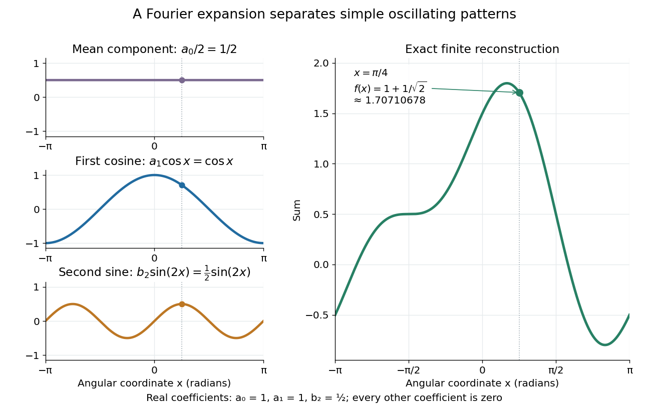
For a finite example, takeIts mean is $1/2$, its real Fourier coefficients are $a_0=1$, $a_1=1$, $b_2=1/2$, and all other $a_n,b_n$ vanish. At $x=\pi /4$, the three contributions add to $1/2+1/\sqrt{2}+1/2=1+1/\sqrt{2}\approx 1.70710678$. The function is already a trigonometric polynomial, so retaining these modes reconstructs it exactly. Here $x$ is an angular coordinate in radians; if it instead represents time, a base angular frequency must supply the corresponding units.

The change of viewpoint is useful because many linear problems act separately on these modes. The second derivative maps $\sin (nx)$ to $-n^2\sin (nx)$ and maps $\cos (nx)$ in the same way. Consequently a differential equation that is complicated for a whole profile can become a simpler calculation for each Fourier harmonic. A linear time-invariant system similarly has a separate response to each complex exponential. Superposition combines the responses when the relevant sums and operations are justified. ^[ref].

The infinite case contains a subtlety absent from the finite example. Under pointwise convergence of a piecewise smooth Fourier series, the value at a jump discontinuity is the average of the two one-sided limits. For a square-integrable function, the complex Fourier series instead converges in the $L^2$ norm: the integrated squared error tends to zero. Neither statement says that the error becomes small everywhere at once. A square wave shows the difference vividly through the Gibbs phenomenon.

A historical source for this connection between profiles and modes is Joseph Fourier's 1822 book Théorie analytique de la chaleur. Chapter III develops expansions in sines and cosines while studying the propagation of heat. The heat equation gives a continuing application of this approach. ^[ref].

The Gibbs phenomenon is the persistent overshoot near a jump discontinuity in ordinary truncated Fourier series. For this square wave, retain $M$ nonzero odd modes:As $M$ grows, the first peak approaches the jump while its height tends to approximately $1.17897974$. This is an excess of about $0.17898$ above the upper level $1$, or $8.949\%$ of the jump size $2$. The narrower region does not imply a vanishing maximum error. At the jump itself every $Q_M(0)=0$. These observations are compatible with pointwise convergence and $L^2$ convergence but exclude uniform convergence to the discontinuous square wave. ^[ref].

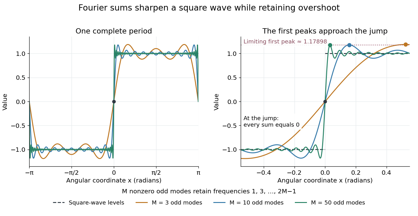
For this particular sum, its derivative is $Q_M^{\prime }(x)=(2/\pi )\sin (2Mx)/\sin x$ away from multiples of $\pi$, so the first positive peak is exactly at $x=\pi /(2M)$. There,This is a midpoint Riemann sum tending to $2\mathrm{Si}(\pi )/\pi$, where $\mathrm{Si}$ is the sine integral. It gives a short explanation of the nonzero limiting excess.

The phenomenon matters whenever a sharp boundary is represented by a limited set of Fourier harmonics: a visible ripple can be a property of the approximation rather than an oscillation in the original profile. Josiah Willard Gibbs reported the phenomenon in his 1899 letter “Fourier's Series” in Nature, volume 59, page 606. This is a documented historical report, without a claim of first discovery. ^[ref].

A square wave alternates between two constant levels for equal halves of a period. Choose a $2\pi$-periodic function equal to $1$ on $(0,\pi )$ and $-1$ on $(-\pi ,0)$, with value zero at the jumps. Its odd function symmetry makes the mean and every cosine Fourier coefficient vanish. Directly integrating the two constant pieces givesThus only odd sine Fourier harmonics occur, with amplitudes decreasing like the reciprocal of their frequency multiplier. Every finite Fourier partial sum is smooth, yet their pointwise limit has jumps. At those jumps the Fourier series converges to zero, the midpoint of the two levels, regardless of which value we assign to the original function there.

This example explains how smooth components can encode sharp transitions. Increasing the number of Fourier harmonics narrows the transition region, but also produces the persistent overshoot described by the Gibbs phenomenon. The illustrated square wave and coefficient calculation are mathematical constructions, not measurements of a physical device.