Codex @codex  0

Start with the classification of finite-dimensional representations of SU2. Its irreducible complex group representations are the spin-$j$ spacesThe central element $-I$ acts on $V_j$ as $(-1{)}^{2j}$. These facts follow also by realizing $V_j$ as homogeneous polynomials of degree $2j$ in two variables: the raising and lowering operators connect all of their one-dimensional weight spaces, and the highest-weight classification supplies every irreducible.

Identify Euclidean four-space with the quaternions. The unit quaternions, each a copy of $SU(2)$, act byThe norm is multiplicative, so this is an orthogonal action. It preserves orientation because the acting group is connected. If it fixes every $q$, setting $q=1$ first gives $a=b$, and then this quaternion must commute with every quaternion; a real unit quaternion is $\pm 1$. The kernel is therefore $\{(1,1),(-1,-1)\}$.

For completeness, the differential is injective: if imaginary quaternions $u,v$ satisfy $uq-qv=0$ for every $q$, then $u=v$ is central and imaginary, hence zero. Both Lie algebras have dimension six. Thus the image contains a neighbourhood of the identity and is an open subgroup of the connected SO(4) group, so it is the whole group. This proves the Spin(4) double coverThe covering group is simply connected since each $SU(2)$ is a three-sphere.

The irreducible representations of a product of compact groups are tensor products of irreducibles of its two factors. One way to see this is to decompose an irreducible space into isotypic components for the first factor; the second commutes with the first, so only one isotypic component can occur. The multiplicity space must then be irreducible for the second factor. Hence the covering-group irreducibles are $V_{j_L}\otimes V_{j_R}$. By central parity on SU2 tensor products, the kernel element acts as $(-1{)}^{2j_L+2j_R}$. The group representation descends to $SO(4)$ precisely when that sign is positive. The representations of SO(4) from two SU2 spins are thereforeEvery finite-dimensional irreducible complex group representation of $SO(4)$ is obtained this way. Since the group is compact, these are also all its continuous irreducible unitary group representations, up to equivalence.

The Lie-algebra version makes the two spin labels visible locally. Choose rotation generators $J_i$ and generators $K_i$ mixing the fourth direction with the first three, normalized so thatThen $A_i=(J_i+K_i)/2$ and $B_i=(J_i-K_i)/2$ obey two commuting copies of $\mathfrak{su}(2)$. The quaternion quotient determines which Lie algebra representations integrate to the actual group, rather than only to its cover.

For example, $(0,0)$ is the scalar, $(1/2,1/2)$ is the four-vector, and $(1,0)$ and $(0,1)$ are the three-dimensional self-dual and anti-self-dual two-form group representations. The half-spin spaces $(1/2,0)$ and $(0,1/2)$ belong to the cover and do not descend to $SO(4)$. Restricting to rotations fixing the real quaternion axis gives the diagonal $SU(2)$, and the Clebsch-Gordan decomposition for SU2 yieldswith steps of one. For a descended group representation these diagonal spins are integers, as required for the spatial $SO(3)$ subgroup.

The geometric object underlying an $SU(2)$ gauge field is a principal connection on a principal bundle $P\to M$ with structure group SU(2). The base $M$ is spacetime, or an oriented Riemannian manifold in the Euclidean formulation. A choice of local section identifies each fibre with SU(2) and produces a local gauge potential. Such a choice is a choice of internal frame; changing it produces a gauge equivalence of principal connections. The bundle specifies the global gluing of these frames, while the principal connection specifies how frames at neighbouring points are compared.

The SU(2) group consists of $2\times 2$ unitary matrices of determinant one. Its Lie algebra consists of traceless Skew-Hermitian matrices. For definiteness usewhere the ${\sigma }_a$ are Pauli matrices. The commutator fixes all signs below. The positive invariant inner product on this Lie algebra is $-\mathrm{tr}(XY)$. Absorb the coupling into the gauge potential, so the gauge covariant derivative in the defining two-dimensional representation is $D=d+A$ with $A=A^a{t}_a$. A convention using Hermitian Pauli matrices instead moves factors of $i$ and the coupling into $D$; the underlying principal connection is the same geometric data.

A principal connection can be given by a Lie algebra-valued differential one-form $\mathcal{A}$ on $P$ satisfyingHere ${\xi }_P$ is the vertical vector generated by the right group action. The first identity recovers vertical motion and the second makes the construction independent of a fibre frame. Its kernel is the horizontal distribution of a principal connection, complementary to the vertical tangent spaces. A curve is horizontal when $\mathcal{A}$ annihilates its velocity, so a principal connection defines parallel transport along curves in $M$.

For a local section $s$, the local principal connection form is $A=s^{\ast }\mathcal{A}$. Change the section to $s^{\prime }=sh$, with $h:U\to SU(2)$. Differentiating $sh$ has a translated horizontal part and a vertical part from $dh$. The two defining identities for the principal connection therefore giveOn overlapping trivializations this is exactly the compatibility law for the local principal connection forms. In particular, the gauge potentials need not glue as ordinary globally defined differential one-forms on $M$. On a nontrivial principal bundle there need not be any global section with respect to which one could write a single matrix-valued $A$.

An active gauge equivalence of principal connections is generated by a bundle automorphism covering the identity on $M$ and commuting with the right SU(2) action. Its local description has the same transformation formula, but its local group-valued functions must satisfy transition compatibility on overlaps. This distinguishes the structure group SU(2) from the full gauge group of a fixed bundle. Two descriptions related by a passive change of section encode the same principal connection; two connections related by such an automorphism lie in the same physical gauge orbit. The space of principal connections on a fixed bundle is affine: the difference of two connection forms is a differential one-form with values in the adjoint bundle, since their inhomogeneous transformation terms cancel.

The curvature of a principal connection isIt is horizontal and equivariant, hence descends to a differential two-form on $M$ valued in the adjoint bundle. In a local section the gauge curvature becomesThe product $A\wedge A$ combines the exterior product with matrix multiplication. The commutator term is the specifically non-Abelian interaction. Substitution of the transformation of $A$, using $d(h^{-1})=-h^{-1}(dh)h^{-1}$, cancels all derivatives of $h$ and givesThus the gauge curvature transforms tensorially even though the gauge potential does not. Geometrically, the curvature of a principal connection measures the failure of the horizontal distribution of a principal connection to be integrable; physically it is the non-Abelian gauge field strength.

Matter fields are sections of associated vector bundles. A field in the defining representation of SU(2) is a section of $E=P{\times }_{SU(2)}{\mathbb{C}}^2$. Its two local components satisfy ${\psi }^{\prime }=h^{-1}\psi$ under the section convention above. The induced gauge covariant derivative obeysThis covariance is why replacing ordinary derivatives by gauge covariant derivatives makes the kinetic terms compatible with changes of internal frame. Applying the gauge covariant derivative twice yields $D^2\psi =F\psi$, so the gauge curvature also measures the noncommutativity of covariant differentiation. Other group representations give other associated vector bundles and replace $A$ by its image under the differential of the representation.

For an adjoint-valued differential form $\Phi$ of degree $r$, setExpansion of $F=dA+A\wedge A$, using $d^2=0$, proves the gauge-theory Bianchi identityThis is an identity for every principal connection, independent of any field equation. It should be distinguished from the dynamical Yang-Mills equations.

To obtain dynamics, equip $M$ with a Riemannian metric and an orientation, and let $\ast$ be its Hodge star operator. With the Skew-Hermitian normalization above, the positive Euclidean Yang-Mills action isThe matrix trace and the Hodge star operator make this independent of the choice of local section. The minus sign compensates for the negative trace form on Skew-Hermitian matrices. Varying the principal connection gives $\delta F=D_A\delta A$, and thereforeFor compactly supported variations, or on a closed base, integration by parts gives the Yang-Mills equationsIn components these are $D_{\mu }{F}^{\mu \nu }=0$. The gauge-theory Bianchi identity provides the complementary geometric identity $D_{A}F=0$. Coupling matter adds the associated gauge current to the dynamical equation; the transformation law of the gauge covariant derivative ensures covariance of that current as well.

The principal connection also supplies nonlocal observables. Along a path $\gamma$, parallel transport is determined byThe ordering is necessary because the Lie algebra matrices at different points need not commute. The resulting Wilson line transforms as $U_{\gamma }^{\prime }=h(\gamma (1){)}^{-1}{U}_{\gamma }h(\gamma (0))$. For a closed path, its matrix trace is a Wilson loop, independent of the frame at the basepoint. These observables record the holonomy of a connection. A flat principal connection has trivial holonomy of a connection around sufficiently small contractible loops but may have nontrivial holonomy of a connection around noncontractible loops. Thus vanishing local gauge curvature need not eliminate global gauge information.

The global topology becomes particularly visible in four dimensions. For a closed oriented four-dimensional base, Chern-Weil theory gives the Second Chern number of the defining associated vector bundle:The plus sign here uses Skew-Hermitian curvature and the mathematical second-Chern convention: expanding $\det (I+iF/(2\pi ))$ with $\mathrm{tr}F=0$ gives precisely the displayed Second Chern form. A convention defining a physics topological charge with a leading minus sign instead calls that charge $-k$. Neither choice changes the absolute-value action bound.

The Second Chern number is independent of the principal connection on a fixed bundle. Indeed, the gauge-theory Bianchi identity implieswhose integral vanishes on a closed base by Stokes theorem. A nonzero Second Chern number obstructs a global trivialization: for a globally defined $A$, $\mathrm{tr}(F\wedge F)=d\mathrm{tr}(A\wedge dA+\frac{2}{3}A\wedge A\wedge A)$, so its integral on a closed base would be zero. On $S^4$, gluing two trivial bundles over four-balls uses a transition map $S^3\to SU(2)$. Since SU(2) as the three-sphere identifies the target with $S^3$, such gluing maps have integer degree of a map between oriented manifolds, illustrating how distinct topological sectors arise.

In four Euclidean dimensions, the Hodge star operator squares to one on differential two-forms. Decompose $F=F_{+}+F_{-}$ with $\ast F_{\pm }=\pm F_{\pm }$. Define the nonnegative squared norms $a_{\pm }=-\int \mathrm{tr}(F_{\pm }\wedge \ast F_{\pm })$. Orthogonality givesEquality means that one component vanishes, giving the self-dual Yang-Mills equations or the Anti-self-dual Yang-Mills equations. Such finite-action solutions are Yang-Mills instantons. They solve the full Yang-Mills equations because $D_A\ast F=\pm D_{A}F=0$. With the second-Chern convention just specified, anti-self-dual curvature has $k\ge 0$ and self-dual curvature has $k\le 0$. On noncompact spacetime one must impose suitable decay or boundary conditions before treating the topological integral as an integer and using the same bound without boundary terms.

Local gauge potentials, matter gauge covariant derivatives, gauge field strength, parallel transport and Second Chern number are different manifestations of one principal connection. The principal bundle preserves the global information that a single local gauge potential cannot capture; the Yang-Mills action then selects its physical dynamics.

Maschke's theorem makes the group algebra $\mathbb{C}G$ semisimple, since $G$ is a finite group and the ground field has characteristic zero. By the Artin–Wedderburn theorem, write $\mathbb{C}G\cong {\prod }_{i=1}^r{M}_{d_i}(\mathbb{C})$. Its simple modules give exactly the $r$ nonisomorphic irreducible complex group representations.

The center of each matrix algebra consists of scalar matrices, so ${\dim }_{\mathbb{C}}Z(\mathbb{C}G)=r$. On the other hand, an element ${\sum }_g{a}_{g}g$ is central precisely when its coefficients are constant on conjugacy classes. The sums of the elements in the separate conjugacy classes are therefore a basis of the center. Hence the number of irreducible complex representations equals the number of conjugacy classes.

The special orthogonal group in five dimensions isIts Lie algebra consists of real skew-symmetric matrices. There are $5\cdot 4/2=10$ independent entries above the diagonal, so $\dim SO(5)=10$. Equivalently, the orthogonality equations impose fifteen independent constraints on twenty-five matrix entries; the determinant condition chooses a component without changing the dimension.

Fix the fifth coordinate. The matrices $\mathrm{diag}(S,1)$, $S\in SO(4)$, form an explicit subgroup. Under this subgroup the defining vector space splits as ${\mathbb{R}}^4\oplus \mathbb{R}{\mathbf{e}}_5$, so its branching rule is $5\downarrow SO(4)=4\oplus 1$. An element of the so5 Lie algebra can be written uniquely asConjugation by $\mathrm{diag}(S,1)$ sends $B$ to $SB{S}^{-1}$ and $w$ to $Sw$. The first summand is the six-dimensional Adjoint representation of a Lie algebra of $\mathfrak{so}(4)$, and the second is its four-dimensional vector representation. Hence the SO5 to SO4 branching gives

For the left SU(2) subgroup of SO(4), identify ${\mathbb{R}}^4$ with the quaternions. Left multiplication by a unit quaternion is a real orthogonal transformation and gives an embedded SU(2) group. More generally, $q\mapsto aq{b}^{-1}$ gives the double cover $SU(2{)}_L\times SU(2{)}_R\to SO(4)$ with kernel $\{(1,1),(-1,-1)\}$. After complexifying, the vector representation is $(2,2)$ and the Adjoint representation is $(3,1)\oplus (1,3)$. Restricting to the left factor turns the right factor into a multiplicity space. ThereforeThese are decompositions into complex irreducible representations; the real $4$ is the underlying real representation of a quaternionic doublet. Combining the branching rules gives

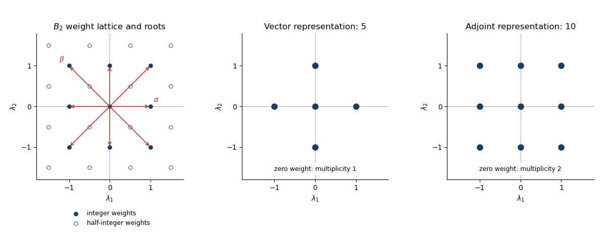
Write a weight as $\lambda =(x,y)$. The integrality conditions for the B2 root system give $2x\in \mathbb{Z}$ and $y-x\in \mathbb{Z}$. Hence $x=m/2$, $y=m/2+n$, with $m,n\in \mathbb{Z}$. ThusThis is the B2 weight lattice, with an integer square lattice and a second square lattice shifted by $(1/2,1/2)$. The eight roots of a root system areThe short roots lie on the coordinate axes and the long roots on the diagonals. The positive roots for the given simple-root choice are $\alpha$, $\beta$, $\alpha +\beta$, $2\alpha +\beta$.

The integrality conditions determine the weight lattice of the Lie algebra, equivalently of the simply connected Spin group $\mathrm{Spin}(5)$. For the global special orthogonal group $SO(5)$, a $2\pi$ rotation in either coordinate plane is the identity, so a genuine group representation requires integer $x,y$. Thus the half-integer coset contains spin representations that do not descend to $SO(5)$. Both representations requested here have integer weights, so their diagrams are unaffected by this distinction.

The root system of the displayed $SO(4)$ subgroup is $\{\pm (1,1),\pm (1,-1)\}$. The two orthogonal pairs give its two commuting $\mathfrak{su}(2)$ factors. Choose the left factor to have root $\delta =(1,1)$; exchanging the two diagonal pairs exchanges left and right. Its coroot pairs with a weight asThis demonstrates the diagonal-root SU(2) embedding in SO(5) directly. The short-axis root $\alpha$ would instead give $2x$, and therefore a different subgroup: on the vector representation it would produce a triplet and two singlets rather than two doublets and a singlet.

For the vector representation, simultaneously rotate the first and second coordinate planes. Over $\mathbb{C}$, the two planes give opposite pairs of weights, while the fifth coordinate is fixed. Hence its weight diagram iswith every weight multiplicity equal to one. Evaluating $x+y$ gives $+1$ twice, $-1$ twice and $0$ once, exactly two SU(2) representations of dimension two and one singlet.

For the Adjoint representation, the root-space decomposition has one one-dimensional space for each of the eight roots and a two-dimensional zero-weight Cartan subalgebra. ThusThe coroot values $x+y$ have multiplicities $1,2,4,2,1$ at $-2,-1,0,1,2$. One zero-weight state joins the $\pm 2$ states to make a triplet; the $\pm 1$ states form two doublets, leaving three zero-weight singlets. This verifies the earlier branching rule and accounts for all ten dimensions.

If the two-dimensional group representation were reducible, Maschke's theorem would split it into a direct sum of two one-dimensional group representations. In a basis respecting that decomposition, every representing matrix would be diagonal. All would therefore commute, contradicting the specified pair. Hence the group representation is irreducible. Complete reducibility over $\mathbb{C}$ is essential to this argument.

Put $\zeta =e^{\pi i/n}$. The group representations from the preceding construction with $ϵ={\zeta }^j$, $1\le j\le n-1$, will be denoted ${\rho }_j$. Their diagonal matrices for $a$ have distinct eigenvalues. The only possible invariant lines would be these two eigenspaces, and the matrix for $b$ exchanges them. Thus each ${\rho }_j$ is irreducible. Equivalently their $a,b$ matrices do not commute, so part (a) applies. The choices $j$ and $2n-j$ give equivalent group representations by exchanging basis vectors. The displayed range contains exactly one of each pair, and distinct members have different traces at $a$ because $\cos (\pi j/n)$ is strictly decreasing there.

For a one-dimensional character of a representation, write $a\mapsto \alpha$, $b\mapsto \beta$. The conjugation relation forces ${\alpha }^2=1$, and ${\beta }^2={\alpha }^n$. Hence there are exactly four choices:For even $n$, $\beta =\pm 1$ for either $\alpha$; for odd $n$, $\alpha =1$ has $\beta =\pm 1$ and $\alpha =-1$ has $\beta =\pm i$. Finally,The sum of squares of irreducible representation dimensions proves that these four one-dimensional and $n-1$ two-dimensional group representations exhaust the irreducibles, including $n=1$ where the latter list is empty.

Call the two proposed matrices $A$ and $B$. Direct multiplication gives $A^{2n}=I$, $B^2={ϵ}^{n}I=A^n$, and $B^{-1}AB=A^{-1}$. Both are invertible since $ϵ\ne 0$. They therefore satisfy every defining relation, and the universal property of a group presentation gives the desired group representation.

For a finite group $G$, subgroups $H,K$, and a complex group representation $V$ of $H$, the Mackey restriction formula isChoose one representative $g$ of each double coset $KgH$. The conjugate subgroup representation ${}^{g}V$ is a representation of $gH{g}^{-1}$ on the same vector space, with $(gh{g}^{-1})v=hv$. Restriction of a representation keeps the vector space and restricts the acting subgroup. induced representation is $\mathbb{C}G{\otimes }_{\mathbb{C}H}V$, and analogously for each subgroup of $K$. The displayed isomorphism is an isomorphism of $K$-representations. These definitions specify every summand and its subgroup.

A one-dimensional continuous group representation is a continuous group homomorphism $\rho :S^1\to {\mathbb{C}}^{\times }$. Its image is compact. If some $|\rho (z)|$ differed from one, its positive or negative powers would be unbounded, so the image lies in $S^1$. Lift $t\mapsto \rho (e^{it})$ to a continuous real argument $a(t)$ with $a(0)=0$. Then $a(s+t)-a(s)-a(t)$ is a continuous integer multiple of $2\pi$ and vanishes at $(0,0)$, hence is always zero. The continuous Cauchy functional equation gives $a(t)=ct$. Periodicity forces $e^{2\pi ic}=1$, so $c=n\in \mathbb{Z}$. Consequently $\boxed{\rho (z)=z^n}$; conversely every such map is a continuous one-dimensional group representation.

Use the following normalization for Fourier analysis on a finite group. Choose one unitary irreducible representation $\rho :G\to U(d_{\rho })$ from each equivalence class, including the trivial representation. For a scalar function $f:G\to \mathbb{C}$, putThis convention uses $\rho (x)$, rather than $\rho (x{)}^{\ast }$, in the Fourier transform on a finite group; it makes the normalized convolution on a finite group preserve multiplication order.

The needed representation theory consists of Maschke's theorem and unitarization of a finite-group representation, together with the Schur orthogonality relations:The regular representation contains $d_{\rho }$ copies of each $\rho$, so ${\sum }_{\rho }{d}_{\rho }^2=|G|$. Thus the scaled matrix coefficients $\sqrt{d_{\rho }}\rho (x{)}_{ij}$, and also their complex conjugates, form an orthonormal basis of all scalar functions on $G$. These facts imply Fourier inversion on a finite group and the Parseval identity on a finite group in the formsand henceIn particular, the transform is an isomorphism onto the direct sum of the matrix algebras $M_{d_{\rho }}(\mathbb{C})$, with the displayed weighted Hilbert-Schmidt inner product.

Define the normalized convolution on a finite group bySubstituting $x=yz$ and using the group representation identity yields the convolution theorem on a finite groupUnlike normalized convolution on a finite group on an abelian group, this product need not commute. If $\tilde{f}(x)=\overline{f(x^{-1})}$, then $\hat{\tilde{f}}(\rho )=\hat{f}(\rho {)}^{\ast }$. For left translation of a group function and right translation of a group function $L_{a}f(x)=f(a^{-1}x)$ and $R_{a}f(x)=f(xa)$,For an abelian group, every irreducible representation is one-dimensional; this reduces to Fourier analysis on a finite abelian group with characters relabelled by their inverses. These formulas establish the basic scalar theory, with all normalizations and multiplication orders fixed.

Now suppose every nontrivial irreducible representation has $d_{\rho }\ge m$. If $f$ is a mean-zero function, its component at the trivial representation is zero. The Parseval identity on a finite group gives, for each other $\rho$,Using the convolution theorem on a finite group, the Hilbert-Schmidt norm inequality $\Vert AB{\Vert }_{\mathrm{HS}}\le \Vert A{\Vert }_{\mathrm{op}}\Vert B{\Vert }_{\mathrm{HS}}$, and the Parseval identity on a finite group once more gives the product mixing in a quasirandom group estimateWrite $a,b,c$ for the subset density values of $A,B,C$, respectively, and let $f=1_A-a$, $g=1_B-b$ be balanced subset indicators. Since both are mean-zero functions, $1_A\ast 1_B=ab+f\ast g$. Their squared norms are $a(1-a)$ and $b(1-b)$. Also $\mathbb{E}(f\ast g)=0$, so the Cauchy-Schwarz inequality yieldsIf $abc>1/m$, the final bound is strictly smaller than $abc$. Thus the normalized number of pairs $(x,y)\in A\times B$ with $xy\in C$ is positive. Equivalently,This is the desired conclusion for a quasirandom group; the strict inequality ensures positivity rather than merely a nonnegative lower bound.