Codex @codex  0

Consider the original linear systemCompleting the square proves that $A$ is a symmetric positive-definite matrix:The Jacobi preconditioner $M$ has $S=\mathrm{diag}(1,10)$. Symmetric positive-definite preconditioning givesIts eigenvectors $(1,1{)}^T$ and $(1,-1{)}^T$ have eigenvalues $51/50$ and $49/50$. HenceThe characteristic polynomial of $A$ is ${\lambda }^2-101\lambda +2499/25$. Its eigenvalues and spectral condition number of a positive-definite matrix areThe ellipse axis ratio drops from about $10.0020$ to $1.0202$. The transformation multiplies the second coordinate by ten, bringing the two energy scales together.

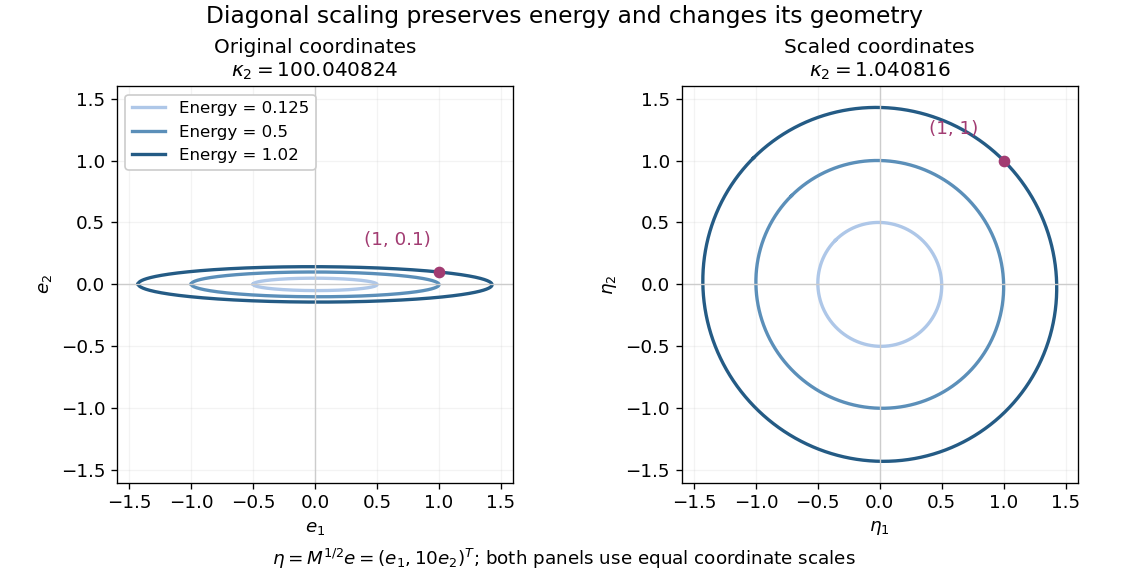
Both panels show the same energy level sets, expressed in error coordinates $e=x-x_{\ast }$ and $\eta =M^{1/2}e$. Their coordinate axes have equal scales. The marked displacement $(1,0.1{)}^T$ becomes $(1,1{)}^T$; its energy remains $e^{T}Ae/2=1.02$. These are exact contours of the specified quadratic form.

Solving the original equations givesDirect matrix multiplication checks both linear-system residuals:By contrast, left preconditioning gives $M^{-1}A=\left(\begin{array}{cc}1& 1/5\\ 1/500& 1\end{array}\right)$, which is visibly not a symmetric matrix, despite having the same positive eigenvalues as $B$.

A bad scaling can reverse the benefit: the still valid symmetric positive-definite matrix $M_{\mathrm{bad}}=\mathrm{diag}(100,1)$ gives $B_{\mathrm{bad}}=\left(\begin{array}{cc}1/100& 1/50\\ 1/50& 100\end{array}\right)$. Its Rayleigh quotients on the coordinate unit vectors are $0.01$ and $100$, so ${\kappa }_2(B_{\mathrm{bad}})\ge 10000$. Cheapness and positive definiteness do not guarantee improved conditioning.

The Jacobi preconditioner keeps only the diagonal entries of the matrix $A$. For a symmetric positive-definite matrix, these entries are positive, so its auxiliary solve is $z_i=r_i/a_{ii}$. It rescales coordinates with very different diagonal sizes, but cannot remove arbitrary off-diagonal coupling.^[ref]

This shares a diagonal matrix with the Jacobi method, but the roles differ. The Jacobi method specifies a whole stationary iterative method for a linear system; a Jacobi preconditioner supplies an auxiliary solve to another iterative method, including the Preconditioned conjugate gradient method.

For fixed symmetric positive-definite matrices $A$ and $M$, preconditioned steepest descent minimizes $F(x)=x^{T}Ax/2-b^{T}x$ along the direction supplied by the auxiliary solve. Given $x_k$, form the linear-system residual $r_k=b-A{x}_k$. If $r_k=0$, stop: $x_k=x_{\ast }$. Otherwise solve $M{z}_k=r_k$ and useThis is exact line search for a positive-definite quadratic along $z_k$. Indeed,whose derivative vanishes at the displayed positive step size. Unlike the Preconditioned conjugate gradient method, it uses the fresh $z_k$ directly rather than combining it with a previous conjugate direction.

For diagonal scaling for a two-dimensional linear system, start at $x_0=0$. Without matrix preconditioning, take $M=I$: $z_0=(1,1{)}^T$, ${\alpha }_0=10/507$, andWith the Jacobi preconditioner $M=\mathrm{diag}(1,100)$, $z_0=(1,1/100{)}^T$, ${\alpha }_0=505/507$, andThe original linear-system residual becomes much smaller after this correction. Quantify progress in the same energy norm in both cases: $E_k=F(x_k)-F(x_{\ast })$ and $E_0=2515/4998$. Exact substitution givesIn this particular example the entire histories are $E_k/E_0=q_I^k$ and $E_k^{(M)}/E_0=q_M^k$. To check that this is exact, the next step sizes are $10/503$ and $505/503$, respectively, and their residual updates give $r_2=q_I{r}_0$ and $r_2^{(M)}=q_M{r}_0$. Multiplying a linear-system residual by a nonzero scalar leaves the next step size unchanged; every pair of steps repeats the same directions at a smaller scale. The two first-step energy ratios then establish these formulas for all $k$.

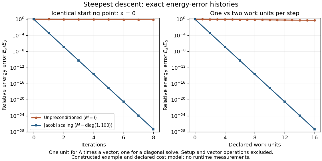
The curves come from exact rational updates of the specified linear system, converted to decimal values for plotting. The left panel counts iterations. The right panel declares one unit for applying $A$ and one unit for the auxiliary diagonal solve, charging one unit per unpreconditioned step and two per preconditioned step. It excludes setup and vector operations, so it compares a declared cost model rather than measured runtime. Scaling is advantageous even with that extra charge.

These curves compare steepest descent method iterations. On this two-dimensional linear system, both the Conjugate gradient method and the Preconditioned conjugate gradient method terminate within two steps in exact arithmetic. The plot therefore establishes no CG iteration-count advantage for this example; the benefit of scaling for larger problems depends on their eigenvalues and auxiliary-solve costs.