A nonnegative regression kernel supplies weights in a local weighted least squares fit. Unlike a probability density function, its integral need not equal one, because rescaling every weight does not change the fitted coefficients.
A smoothing bandwidth determines the scale over which a regression kernel averages data, or a kernel for density estimation spreads each observation. It has the same units as the observations. In kernel density estimation, changing changes the visible detail while preserving the total integral one. For a Gaussian density kernel, each bump has standard deviation and its individual contribution has peak height .
If the smoothing bandwidth is too small relative to the spacings in a statistical sample, the kernel density estimator shows narrow spikes tied to individual observations: apparent peaks may be sampling accidents. If it is too large relative to features of the unknown probability density function, it blurs distinct groups together and spreads fitted probability far from the observations. An intermediate smoothing bandwidth can reveal broad structure, but visual smoothness alone cannot establish accuracy.
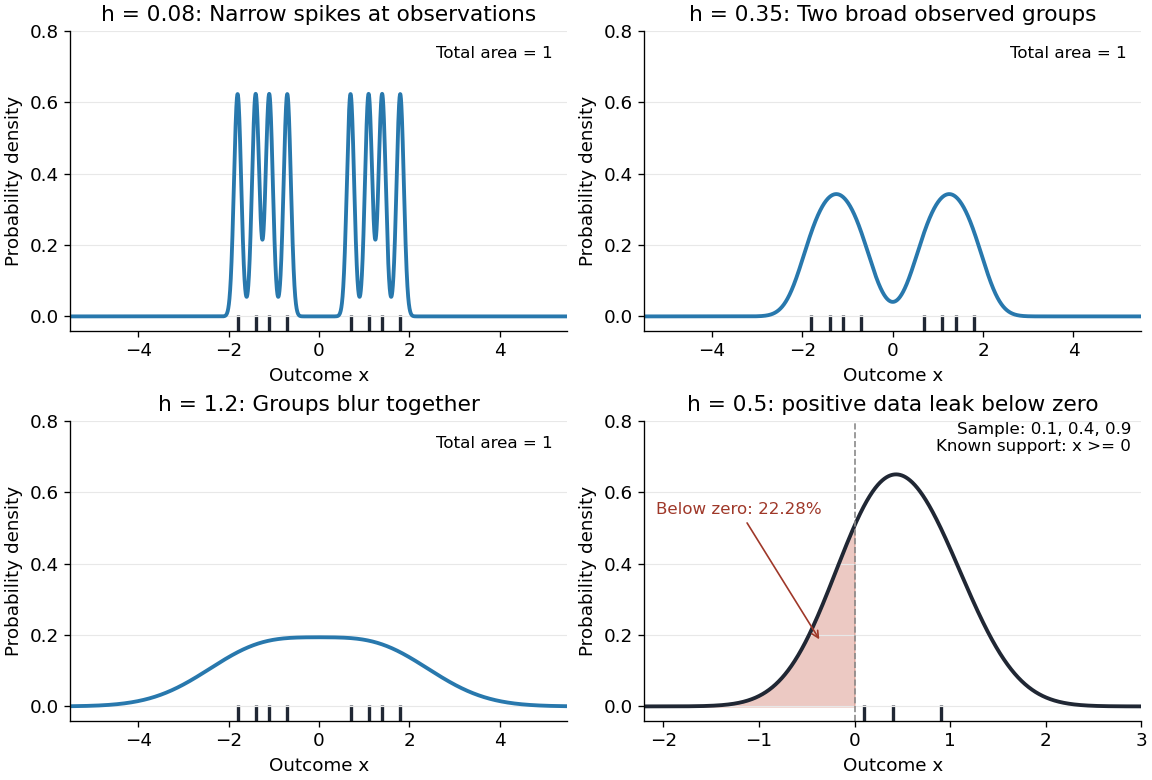
The same sample at three Gaussian bandwidths, and leakage below zero for a separate positive sample
. Details. 
The first three panels use exactly with smoothing bandwidths , and , respectively. Every curve has area one; the two groups in the observed statistical sample become less distinct as increases. No true probability density function is specified in this illustration, so the middle panel is illustrative, not a certified optimal fit. The fourth panel uses and to illustrate boundary bias of a kernel density estimator.
For a fixed nonnegative kernel for density estimation with finite squared integral, a probability density function that is bounded and continuous at an interior point with , and a deterministic sequence , the pointwise sampling variance obeysThus decreasing the smoothing bandwidth increases the leading sampling variance while reducing interior smoothing bias of an estimator: this is a bias-variance tradeoff. The conditions and express two goals, increasingly fine resolution and enough observations contributing locally. Practical methods such as plug-in bandwidth selection use the data to choose ; pointwise optimal kernel bandwidth depends on local features of the unknown probability density function. The smoothing bandwidth remains a tuning choice in nonparametric statistics, and knowing the support of a probability distribution can require more than a width adjustment near a boundary.
Estimate the unknown curvature in the AMISE minimizer and substitute it into that formula. A consistent positive curvature estimate makes the selected bandwidth ratio-consistent. Pilot smoothing is needed because differentiating an undersmoothed density estimator magnifies variance. A normal-reference pilot can initialize an estimate of a higher derivative functional; the final density-curvature estimate is computed from the data rather than assuming the density is normal.
Twice integrating by parts gives . Estimate this by averaging a fourth-derivative kernel density estimator at the observations. Its expectation contains diagonal term and leading smoothing bias . Balancing them yields pilot scale . With suitable derivatives and tails, the estimation error is bounded by , giving an relative-bandwidth bound after substitution. More carefully calibrated bias cancellation can improve that bound.
// Target: statistical-inference.bigb
The uniform smoothing kernel assigns equal weight inside the window and zero weight outside. Its Nadaraya–Watson estimator is the average of observations in that window.
The unit-width centred box kernel is . It has integral one and squared norm one. Its rescaling averages a function on intervals of length . It is obtained from the uniform smoothing kernel with support by rescaling, and is useful in both kernel density estimation and local polynomial regression.
Articles by others on the same topic
There are currently no matching articles.